
Affine Transformation from Fundamental Matrix and Two Directions
Nghia Le Minh
a
and Levente Hajder
b
Department of Algorithms and Their Applications, E
¨
otv
¨
os Lor
´
and University,
P
´
azm
´
any P
´
eter stny. 1/C, H-1117, Budapest, Hungary
Keywords:
Affine Transformation, Epipolar Geometry, Surface Normal Reconstruction, 3D Reconstruction.
Abstract:
Researchers have recently shown that affine transformations between corresponding patches of two images
can be applied for 3D reconstruction, including the reconstruction of surface normals. However, the accurate
estimation of affine transformations between image patches is very challenging. This paper mainly proposes
a novel method to estimate affine transformations from two directions if epipolar geometry of the image pair
is known. A reconstruction pipeline is also proposed here in short. As side effects, two proofs are also given.
The first one is to determine the relationship between affine transformations and the fundamental matrix, the
second one shows how optimal surface normal estimation can be obtained via the roots of a cubic polynomial.
A visual debugger is also proposed to validate the estimated surface normals in real images.
1 INTRODUCTION
Stereo vision has been intensively researched for
many decades in computer vision (Hartley and Zisser-
man, 2003). Classical approaches assume that there
are point correspondences in two images, and then the
3D geometry of the scene and the camera parameters
can be reconstructed. However, it is preferred if the
cameras are calibrated, i.e. the case when the intrin-
sic camera parameters are estimated e.g. by the well-
known chessboard-based method of Zhang (Zhang,
2000).
Recently, researchers have started to process the
affine transformations between corresponding image
patches, not only the corresponding point locations.
A local affine transformation represents the warp be-
tween the infinitely close area around the correspond-
ing point pairs. It can be applied for homography
estimation (Barath et al., 2016), surface normal re-
construction (K
¨
oser and Koch, 2008; Barath et al.,
2015); recovery of epipoles (Bentolila and Francos,
2014), camera pose estimation (K
¨
oser, 2009) as well
as structure-from-motion pipelines (Raposo and Bar-
reto, 2016; Hajder and Eichhardt, 2017).
The input of these algorithms are local affine
transformations. There are many implementations
for detecting the local affinities (Mikolajczyk et al.,
2005). Maybe the most effective ones are affine-
a
https://orcid.org/0000-0001-7690-6245
b
https://orcid.org/0000-0001-9716-9176
covariant feature detectors such as Affine-SIFT
(Morel and Yu, 2009) or Hessian-Affine (Mikolajczyk
and Schmid, 2002).
The goal of this paper is to show that local
affine transformations can be estimated from direc-
tions around point correspondences. The proposed al-
gorithm is theoretically based on the work of Barath
et al. (Barath et al., 2017). They showed that a fun-
damental matrix gives two constraints for an affine
transformation. Their result is exactly the same as
the one published in the work of Raposo and Bar-
reto (Raposo and Barreto, 2016), however, their proof
has geometric meaning. It is demonstrated here that
the other two degrees of freedom (DoF) can be deter-
mined by two corresponding directions of the images.
Contribution. The main theoretical contribution of
the paper is four-fold: (i) First, the proof of (Barath
et al., 2017) is reformulated for the sake of easier un-
derstanding. (ii) Then it is shown that an affine trans-
formation can be estimated from two corresponding
directions in the images if the fundamental matrix of
the stereo setup is known. A linear method is intro-
duced here. (iii) It is shown that the surface normal
can be estimated if the intrinsic camera parameters are
known. Barath et al. (Barath et al., 2015) showed that
the optimal solution can be given via a quartic poly-
nomial, we correct it here and prove that that poly-
nomial is cubic. (iv) It is also demonstrated in the
experiments that affine transformations can be calcu-
lated from optical flow, and these transformations can
be inserted into the reconstruction pipeline.
Minh, N. and Hajder, L.
Affine Transformation from Fundamental Matrix and Two Directions.
DOI: 10.5220/0009154408190826
In Proceedings of the 15th International Joint Conference on Computer Vision, Imaging and Computer Graphics Theory and Applications (VISIGRAPP 2020) - Volume 4: VISAPP, pages
819-826
ISBN: 978-989-758-402-2; ISSN: 2184-4321
Copyright
c
2022 by SCITEPRESS – Science and Technology Publications, Lda. All rights reserved
819

2 AFFINE TRANSFORMATIONS
AND EPIPOLAR GEOMETRY
Given two patches, the centers are p
1
and p
2
, the
affine transformation between the shapes is
A =
a
1
a
2
a
3
a
4
. (1)
The epipolar geometry is represented by the fun-
damental matrix F. As it is well-known in computer
vision, it can be estimated from at least seven point
correspondences (Zhang, 1998).
The stereo problem is visualized in Fig. 1. The
corresponding epipolar lines are as follows:
l
2
= F
p
1
1
,
l
1
= F
T
p
2
1
.
The line normals, i.e. the perpendicular direction
of the lines, are computed as
n
1
=
ˆ
l
1
q
ˆ
l
T
1
ˆ
l
1
=
˜
F
T
"
p
2
1
#
˜
F
T
"
p
2
1
#
2
,
n
2
=
ˆ
l
2
q
ˆ
l
T
2
ˆ
l
2
=
ˆ
F
"
p
1
1
#
ˆ
F
"
p
1
1
#
2
.
where
ˆ
l denotes the first two coordinates of line
parameters, represented by vector x, matrices
˜
F and
ˆ
F consist of the first (left) two columns and (top) two
rows of the fundamental matrix F, respectively.
Points p
1
and p
2
lie on l
1
, and l
2
, respectively.
Therefore, l
T
1
p
1
= 0 and l
T
2
p
2
= 0.
If another point q
1
= p
1
+ εn
1
is taken in the first
image, where n
1
is the normal vector of line l
1
, then
the corresponding epipolar line in the other image is
l
0
2
= F
p
1
1
+ F
εn
1
0
.
The distance d of the original point p
2
and l
0
2
is
d =
p
2
1
T
l
0
2
q
ˆ
l
2
0T
ˆ
l
2
0
,
where
ˆ
l
0
2
is the first two coordinates of line parameters
l
0
2
. Thus
ˆ
l
0
2
=
ˆ
F
p
1
1
+
εn
1
0
.
The denominator is as follows:
q
ˆ
l
2
0T
ˆ
l
2
0
=
ˆ
F
p
1
1
+
εn
1
0
2
.
After elementary modifications, the formula for
distance d can be written as follows:
d =
p
2
1
T
F
p
1
1
+ F
εn
1
0
ˆ
F
p
1
1
+
εn
1
0
2
=
ε
p
2
1
T
F
n
1
0
ˆ
F
p
1
1
+
εn
1
0
2
,
since
p
2
1
T
F
p
1
1
= 0. Therefore,
d = ε
p
2
1
T
˜
Fn
1
ˆ
F
p
1
1
+
εn
1
0
2
.
The scale of the problem can be calculated by
moving the points to infinitely close to the original
position p
1
. Then,
s = lim
ε→0
d
ε
= lim
ε→0
p
2
1
T
˜
Fn
1
ˆ
F
p
1
1
+
εn
1
0
2
=
p
2
1
T
˜
F
˜
F
T
h
p
2
i
˜
F
T
"
p
2
1
#
2
ˆ
F
p
1
1
2
=
p
2
1
T
˜
F
˜
F
T
p
2
1
˜
F
T
p
2
1
2
ˆ
F
p
1
1
2
=
˜
F
T
p
2
1
2
2
˜
F
T
p
2
1
2
ˆ
F
p
1
1
2
=
˜
F
T
p
2
1
2
ˆ
F
p
1
1
2
.
An affinity transforms the normal of an epipolar
line as A
T
n
2
= sn
1
, where s is the scale. This scale
can be eliminated by forcing the directions to be unit
size.
VISAPP 2020 - 15th International Conference on Computer Vision Theory and Applications
820
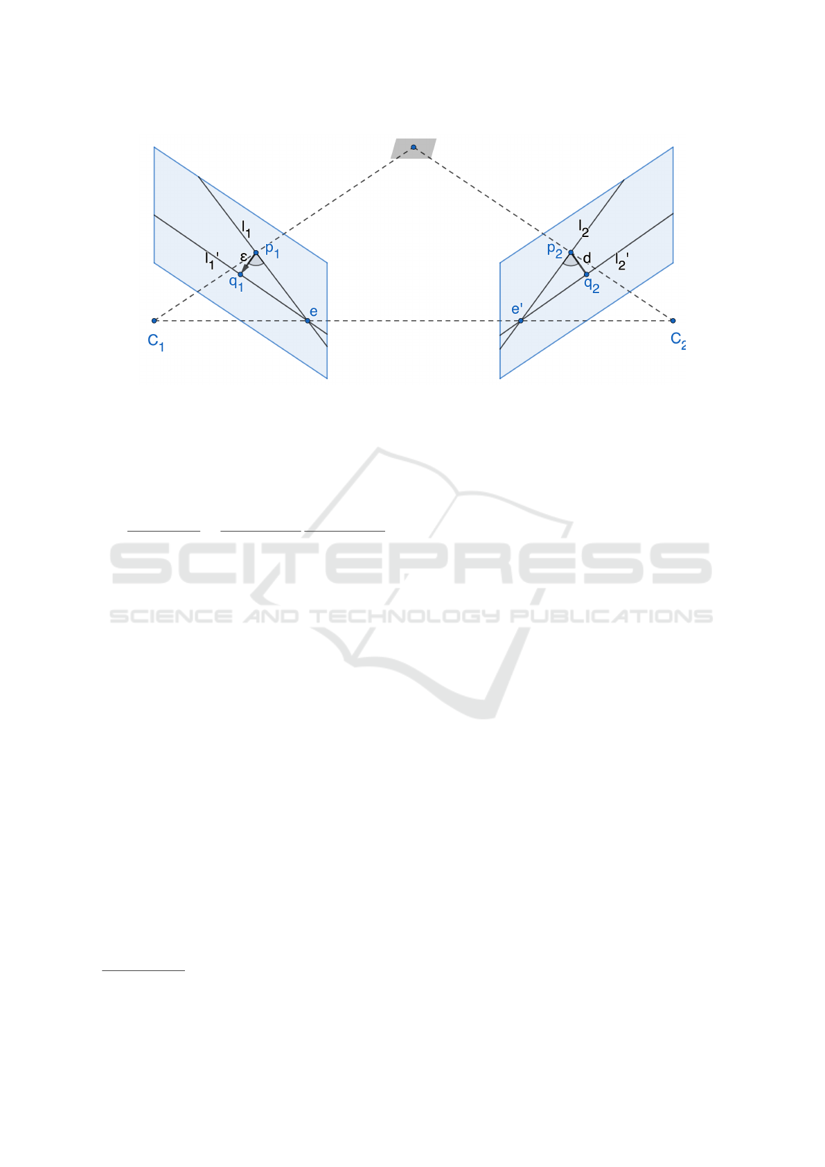
Figure 1: Basic stereo problem for scale estimation. Corresponding point pairs are (p
1
,p
2
) and (q
1
,q
2
); corresponding lines
denoted by (l
1
,l
2
) and (l
0
1
,l
0
2
). The scale to be calculated is given by the ratio d/ε.
If the scale is substituted, and the length of the
normals of epipolar lines are forced to be one, the fol-
lowing equation is obtained:
A
T
ˆ
F
p
1
1
ˆ
F
p
1
1
2
=
˜
F
T
p
2
1
2
ˆ
F
p
1
1
2
˜
F
T
p
2
1
˜
F
T
p
2
1
2
.
The final formula that connects fundamental ma-
trix, point locations and affine correspondences is as
follows
A
T
ˆ
F
p
1
1
= −
˜
F
T
p
2
1
. (2)
The minus sign comes from the fact that the cross
product matrix is a skew-symmetric one and the de-
terminant of the camera matrices have the same sign
1
.
This formula states that a 2D vector equation can be
written for a valid affine transformation if the epipo-
lar geometry, represented by the fundamental matrix,
is known.
3 ESTIMATION OF AN AFFINE
TRANSFORMATION IF
EPIPOLAR GEOMETRY IS
KNOWN
The goal of this section is to show how an affinity
can be estimated for a stereo correspondence if the
1
In other words, both image coordinate systems are left
or right handed.
locations and two corresponding directions are given
in the images. The locations in the images are de-
noted by p
1
=
u
1
v
1
T
and p
2
=
u
2
v
2
T
,
while the directions by d
1i
=
u
1i
v
1i
T
and d
2i
=
u
2i
v
2i
T
,i ∈
{
1,2
}
. The affine transformation is
written by a 2 ×2 matrix as it is defined in Equation 1.
3.1 Estimation of an Affine
Transformation
The relationship between point locations, affine trans-
formation, and the fundamental matrix is given in
Eq. 2. Substituting the coordinates, the following for-
mula is obtained:
A
T
˜
F
u
1
v
1
1
= −
ˆ
F
T
u
2
v
2
1
As the multiplication of the fundamental matrix
and point locations gives the epipolar line in the sec-
ond image, and the transpose of the fundamental ma-
trix and second point location yield the correspond-
ing epipolar line in the first image, the vector-equation
can be rewritten as
A
T
l
2u
l
2v
= −
l
1u
l
1v
,
where the normals of the epipolar lines are the vectors
n
1
= [l
1u
l
1v
]
T
and n
2
= [l
2u
l
2v
]
T
.
If the elements of the affine transformations are
substituted, the following linear system of equations
is given:
a
1
a
3
a
2
a
4
l
2u
l
2v
= −
l
1u
l
1v
. (3)
Affine Transformation from Fundamental Matrix and Two Directions
821

Now the connection between the known directions
is written in conjunction with the affine parameters.
The directions are correctly transformed by the affine
matrix, however, the lengths of the vectors are not
known. This fact can be formulated as
A
u
11
v
11
= α
1
u
21
v
21
,
A
u
12
v
12
= α
2
u
22
v
22
,
where α
1
and α
2
are the unknown lengths.
It can be straightforwardly rewritten by substitut-
ing the elements of the affine transformations as
a
1
a
2
a
3
a
4
u
11
v
11
= α
1
u
21
v
21
,
a
1
a
2
a
3
a
4
u
12
v
12
= α
2
u
22
v
22
. (4)
The final problem can be formed by merging
Equations 3 and 4. The problem is a six-dimensional
linear one, it is written in Equation 5. The solution
is trivially obtained by multiplying the right vector by
the inverse of the coefficient matrix from the left.
3.2 Affine Transformation from Optical
Flow
The affine transformations can be estimated by other
techniques, e.g. using an affine-invariant matcher (Yu
and Morel, 2011). However, from our experience, the
quality of those are not satisfactory, because the esti-
mated transformations are highly contaminated.
We have tried another way: the affine transforma-
tions are estimated if the optical flow between the im-
ages is available. The estimation problem is an in-
homogeneous linear one as it is discussed in the ap-
pendix. Therefore, the estimation is very fast, the
pseudo-inverse of a matrix, corresponding to a 6D
problem, has to be computed.
Problem Statement. An optical flow is given, thus
the relative offset for each camera pixels are known
as
x
0
i
y
0
i
=
x
i
y
i
+
∆x
i
∆y
i
,
where the vector [x
i
y
i
]
T
and [x
0
i
y
0
i
]
T
denote the
pixel coordinates in the first and second images, re-
spectively. The flow itself is represented by the offset
vectors [∆x
i
∆y
i
]
T
.
The task is to estimate the affine transformation
around the given point location x
0
= [x
0
,y
0
].’Around’
means that the neighbouring pixels has to be consid-
ered. they are selected in a disk with radius R, where
R is a parameter of the algorithm.
Proposed Solution. The affine transformation repre-
sents the relations between corresponding neighbour-
ing points as
x
0
i
y
0
i
=
a
1
a
2
a
5
a
3
a
4
a
6
x
i
y
i
1
.
Thus,
x
0
i
y
0
i
=
a
1
a
2
a
3
a
4
x
i
y
i
+
a
5
a
6
.
In other form:
x
i
y
i
1 0 0 0
0 0 0 x
i
y
i
1
a
1
a
2
a
5
a
3
a
4
a
6
=
x
0
i
y
0
i
.
Left matrix is denoted by C
i
. then
C
i
a
1
a
2
a
5
a
3
a
4
a
6
T
= x
0
i
.
If we have N different locations, the problem is over-
determined:
C
1
C
2
.
.
.
C
N
a
1
a
2
a
5
a
3
a
4
a
6
=
x
0
1
x
0
2
.
.
.
x
0
N
It should be considered for all pixels that fulfill
the constraint (x
0
− x
i
)
T
(x
0
− x
i
) < R
2
. The problem
is linear:
C
a
1
a
2
a
5
a
3
a
4
a
6
T
= x
0
,
where C = [C
T
1
... C
T
N
]
T
and x = [x
T
1
... x
T
N
]
T
. The op-
timal solution for the affine parameters are estimated
as follows:
a
1
a
2
a
5
a
3
a
4
a
6
T
=
C
T
C
−1
C
T
x
0
.
Remark that optical flow for at least three loca-
tions is required. With more than three points the
problem is over-determined.
VISAPP 2020 - 15th International Conference on Computer Vision Theory and Applications
822

l
2u
0 l
2v
0 0 0
0 l
2u
0 l
2v
0 0
u
11
v
11
0 0 −u
21
0
0 0 u
11
v
11
−v
21
0
u
12
v
12
0 0 0 −u
22
0 0 u
12
v
12
0 −v
22
a
1
a
2
a
3
a
4
α
1
α
2
=
−l
1u
−l
1v
0
0
0
0
(5)
4 OPTIMAL SURFACE NORMAL
ESTIMATION
In this section, we prove that the polynomial, defined
in (Barath et al., 2015) is cubic and not quartic.
If we restrict the estimating normal into the form
n = [x,y,1 − x − y]
T
(i.e the sum of coordinates is 1),
then the roots of the mentioned polynomial are the
possible values of x.
The notations come from the original paper
2
. Un-
fortunately, the full proof cannot be repeated here due
to the page limit of the submission.
The coefficients for the polynomials are deter-
mined by the point locations in the stereo image pair
and the related affine transformation.
The initial facts for our proof is that the following
rules can be formed:
Ω
1
k
= Ψ
2
k
= 0, Ω
2
k
= −Ψ
1
k
,
as it is written in page 21 of the paper (Barath
et al., 2015).
Then the coefficients for the quadratic curves are
as follows
3
:
A
2
=
4
∑
k=1
Ω
k
Ω
2
k
, B
1
=
4
∑
k=1
Ψ
k
Ψ
1
k
C
1
=
4
∑
k=1
(Ω
1
k
Ψ
k
+ Ψ
1
k
Ω
k
) =
4
∑
k=1
Ψ
1
k
Ω
k
C
2
=
4
∑
k=1
(Ω
2
k
Ψ
k
+ Ψ
2
k
Ω
k
) =
4
∑
k=1
Ω
2
k
Ψ
k
Coefficient for x
4
, i.e. the highest one of the poly-
nomial, is as follows:
A
2
2
B
1
− A
2
C
1
C
2
= A
2
(A
2
B
1
−C
1
C
2
)
= A
2
(
4
∑
k=1
Ω
k
Ω
2
k
4
∑
k=1
Ψ
k
Ψ
1
k
−
4
∑
k=1
Ψ
1
k
Ω
k
4
∑
k=1
Ω
2
k
Ψ
k
)
2
The proof described here cannot be understood without
reading the original paper. The related part is found in the
appendix of the paper (Barath et al., 2015), however, Sec-
tion 2, i.e. geometric background, has to be read as well.
3
Not all coefficients are listed, only the ones that are
required to understand the proof.
= A
2
(
4
∑
i=1
4
∑
j=1
Ω
i
Ω
2
i
Ψ
j
Ψ
1
j
−
4
∑
i=1
4
∑
j=1
Ψ
1
i
Ω
i
Ω
2
j
Ψ
j
)
= A
2
(
4
∑
i=1
4
∑
j=1
Ω
i
Ω
2
i
Ψ
j
Ψ
1
j
−
4
∑
i=1
4
∑
j=1
Ψ
1
i
Ω
i
Ω
2
j
Ψ
j
)
= A
2
(
4
∑
i=1
4
∑
j=1
Ω
i
(−Ψ
1
i
)Ψ
j
(−Ω
2
j
)−
4
∑
i=1
4
∑
j=1
Ψ
1
i
Ω
i
Ω
2
j
Ψ
j
)
= A
2
(
4
∑
i=1
4
∑
j=1
Ω
i
Ψ
1
i
Ψ
j
Ω
2
j
−
4
∑
i=1
4
∑
j=1
Ψ
1
i
Ω
i
Ω
2
j
Ψ
j
) = 0
Thus, the highest coefficient vanishes, therefore
the degree of the polynomial is three, in other words,
the polynomial is cubic. .
5 RECONSTRUCTION PIPELINE
This section overviews the components of our recon-
struction pieline.
In the first stage, point correspondences are de-
tected using ASIFT (Yu and Morel, 2011). Then the
fundamental matrix is estimated by the eight-point
method (Hartley, 1995). As the cameras are pre-
calibrated, essential matrix can also be retrieved from
fundamental matrix and intrinsic camera parameters.
In order to estimate affine transformations, two
corresponding directions have to be found. First, Line
Segment Detector (von Gioi et al., 2012) and Line Bi-
nary Descriptor (Zhang and Koch, 2013) are applied
to the image patches centered around feature points
so that at least two segment pairs are matched. The
directions are obtained through the normalized direc-
tion vector of those segments. Then affinities are es-
timated from the fundamental matrix and two direc-
tions as discussed in Section 3.
With the feature point locations and the recovered
camera pose
4
, one can compute a sparse 3D recon-
struction. This step is carried out by applying Hartley-
Sturm triangulation (Hartley and Sturm, 1997). Fi-
nally, optimal surface normals can be estimated from
4
Camera extrinsic parameters, i.e. the relative pose, can
be obtained by decomposing the essential matrix (Hartley
and Zisserman, 2003)
Affine Transformation from Fundamental Matrix and Two Directions
823
affine transformations by the proposed modification,
overviewed in Section 4, of the method of Barath et
al (Barath et al., 2015).
6 EXPERIMENTS
For testing, we concentrate mainly on real-world case
as the main goal of our work is to insert the surface
normal estimation into a 3D reconstruction pipeline.
6.1 Synthetic Test
Synthetic test was only constructed in order to vali-
date that the formula, given in Eq. 5, is correct. For
this purpose, a simple synthetic testing environment
was implemented in Octave
5
. Camera parameters as
well as the scene geometry, i.e. a sphere in our en-
vironment, was randomly generated, point locations
were given by projecting the points into the camera
image. Ground-truth affine transformations were gen-
erating via the tangent planes of the sphere. The affine
parameters can be determined by derivating the ho-
mographies, related to the tangent planes, at the corre-
sponding point locations as it is discussed in the paper
of Barath et al. (Barath et al., 2015) in detail.
Conclusion of Synthetic Test. It was successfully
validated that Equation 5 is correct, the GT affine
transformations were always exactly retrieved.
6.2 Visual Debugger
We have developed a tool in order to run the re-
construction pipeline and visualize the computed sur-
face normals. We call this tool as Visual Debug-
ger. The point correspondences as well as the di-
rections are manually selected in order to avoid de-
tection errors. The fundamental matrix is automat-
ically estimated by the eight-point method (Hartley,
1995). Robustification is implemented using the stan-
dard RANSAC (Fischler and Bolles, 1981) scheme.
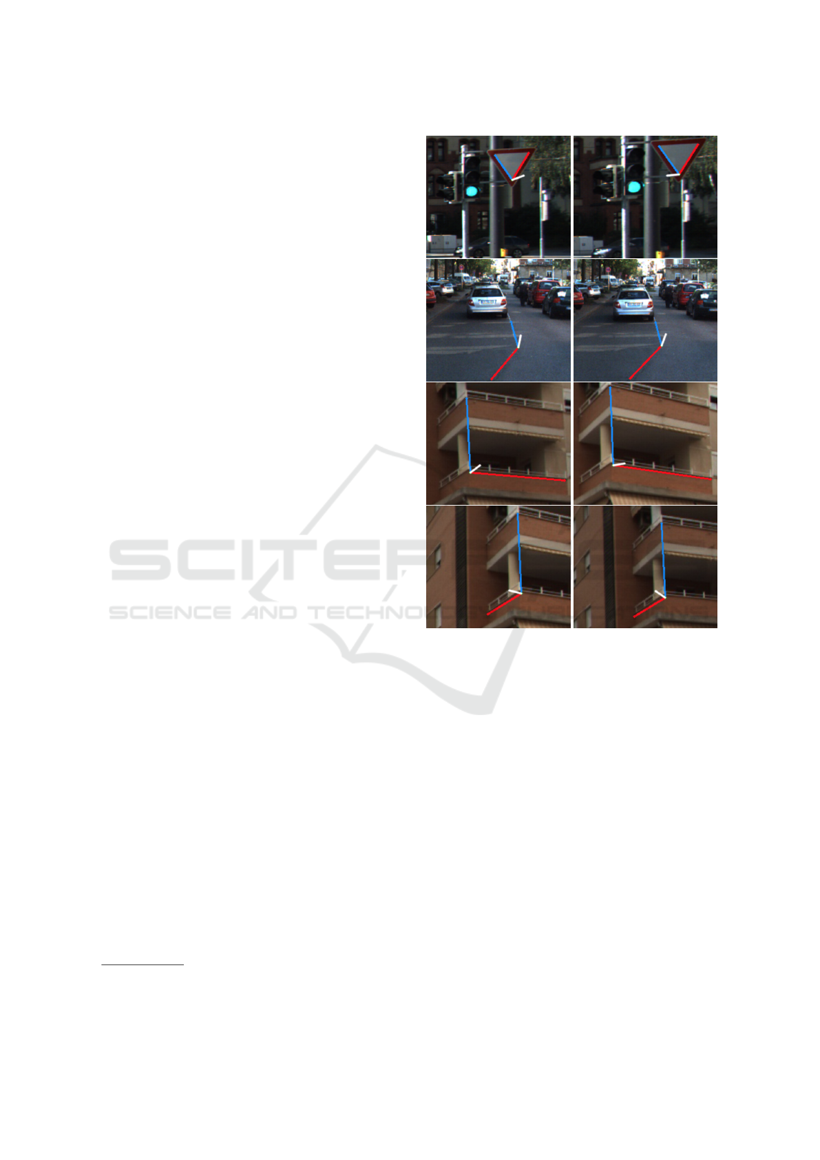
A few results by the Visual Debugger are seen
in Figure 2. We have tested our method on the
KITTI (Geiger et al., 2012) and Malaga (Blanco et al.,
2014) datasets.
6.3 Surface Normals
A fully automatic testing procedure were also carried
out using the whole reconstruction pipeline. An ex-
ample with the visualized normal vectors is pictured
5
Octave is an open-source MATLAB-clone. See
http://www.octave.org.
Figure 2: Results on real sequences. Each row consists of
a stereo image pair. The manually selected directions are
colored by red and blue. The estimated surface normals are
visualized by white. Best viewed in color.
in Figure 3. The normals are differently colored: the
absolute values of the coordinates of the normals are
considered; if the largest absolute coordinate of a vec-
tor is x, y, and z, then yellow, white, and red color is
used for drawing it, respectively.
6.4 Surface Normal Reconstruction
from Optical Flow
Although the focus of this paper is to show that
affine transformations can be estimated from two cor-
responding directions and the fundamental matrix,
we demonstrated here that there are other ways to
efficiently estimate the affine transformations. In
Sec. 3.2, it is overviewed how an transformation can
be retrieved at a given location if the optical flow be-
tween the images is given. The surface normals can be
estimated by the optimal method, proposed in Sec 4.
VISAPP 2020 - 15th International Conference on Computer Vision Theory and Applications
824

Figure 3: Estimated surface normals visualized in an image of one of the KITTI (Geiger et al., 2012) sequences. Yellow,
white and red coordinates are used for horizontal, vertical and perpendicular, to the image plane, directions. Best viewed in
color.
Figure 4: Estimated surface normals visualized in images
generated by simulator LG-SVL (LG-, 2019). Yellow,
white and red coordinates are used for horizontal, vertical
and perpendicular, to the image plane, directions. Affine
transformations are computed from optical flow. Best
viewed in color..
The image sequences were generated by the LG-
SVL Simulator (LG-, 2019). The optical flows were
computed by the pre-trained deep network HD3 (Yin
et al., 2019). Resulting images are visualized in Fig-
ure 4, the estimated surface normals are drawn. Al-
though affine transformations can be estimated for
each pixel location, a regular sparse grid is applied
for sampling due to easier interpretation.
7 CONCLUSIONS AND FUTURE
WORK
In this position paper, we have presented a novel re-
construction pipeline in order to compute the surface
normals of a 3D scene. It has been shown that an
affine transformation can be estimated from a point
and two line (direction) correspondences if the funda-
mental matrix is known. The surface normals them-
selves can be estimated via the roots of cubic polyno-
mials.
Future Work. This paper concentrates on the theo-
retic aspects of the problem. More quantitative and
qualitative tests are required in order to validate the
practical applicability of the proposed reconstruction
pipeline.
The four DoF of affine transformations means that
the knowledge of epipolar geometry and two direc-
tions are enough to estimate a local affine transfor-
mation. However, there are degenerate cases when
a direction and the fundamental matrix represent the
same information for the estimation. These degener-
ate cases have also to be found and discussed. This is
missing in the current form of the paper.
ACKNOWLEDGEMENTS
Nghia Le Minh was supported by the project
EFOP-3.6.3-VEKOP-16- 2017-00001: Talent Man-
agement in Autonomous Vehicle Control Technolo-
gies, by the Hungarian Government and co-financed
by the European Social Fund. Levente Hajder was
supported by the project no. ED 18-1-2019-0030:
Application domain specific highly reliable IT solu-
tions subprogramme. It has been implemented with
the support provided from the National Research, De-
velopment and Innovation Fund of Hungary, financed
Affine Transformation from Fundamental Matrix and Two Directions
825

under the Thematic Excellence Programme funding
scheme.
REFERENCES
(2019). LGSVL Simulator.
https://www.lgsvlsimulator.com/.
Barath, D., Molnar, J., and Hajder, L. (2015). Optimal Sur-
face Normal from Affine Transformation. In VISAPP
2015, pages 305–316.
Barath, D., Molnar, J., and Hajder, L. (2016). Novel meth-
ods for estimating surface normals from affine trans-
formations. In Computer Vision, Imaging and Com-
puter Graphics Theory and Applications, pages 316–
337. Springer International Publishing.
Barath, D., Toth, T., and Hajder, L. (2017). A minimal so-
lution for two-view focal-length estimation using two
affine correspondences. In 2017 IEEE Conference
on Computer Vision and Pattern Recognition, CVPR
2017, Honolulu, HI, USA, July 21-26, 2017, pages
2557–2565.
Bentolila, J. and Francos, J. M. (2014). Conic epipolar con-
straints from affine correspondences. Computer Vision
and Image Understanding, 122:105–114.
Blanco, J.-L., Moreno, F.-A., and Gonzalez-Jimenez, J.
(2014). The m
´
alaga urban dataset: High-rate stereo
and lidars in a realistic urban scenario. International
Journal of Robotics Research, 33(2):207–214.
Fischler, M. and Bolles, R. (1981). RANdom SAmpling
Consensus: a paradigm for model fitting with appli-
cation to image analysis and automated cartography.
Commun. Assoc. Comp. Mach., 24:358–367.
Geiger, A., Lenz, P., and Urtasun, R. (2012). Are we ready
for autonomous driving? the kitti vision benchmark
suite. In Conference on Computer Vision and Pattern
Recognition (CVPR).
Hajder, L. and Eichhardt, I. (2017). Computer vision
meets geometric modeling: Multi-view reconstruction
of surface points and normals using affine correspon-
dences. In 2017 IEEE International Conference on
Computer Vision Workshops, ICCV Workshops 2017,
Venice, Italy, October 22-29, 2017, pages 2427–2435.
Hartley, R. I. (1995). In defence of the 8-point algorithm.
International Conference on Computer Vision, pages
1064–1070.
Hartley, R. I. and Sturm, P. (1997). Triangulation. Computer
Vision and Image Understanding: CVIU, 68(2):146–
157.
Hartley, R. I. and Zisserman, A. (2003). Multiple View Ge-
ometry in Computer Vision. Cambridge University
Press.
K
¨
oser, K. (2009). Geometric Estimation with Local Affine
Frames and Free-form Surfaces. Shaker.
K
¨
oser, K. and Koch, R. (2008). Differential spatial resection
- pose estimation using a single local image feature. In
ECCV, pages 312–325.
Mikolajczyk, K. and Schmid, C. (2002). An affine invariant
interest point detector. In Computer Vision - ECCV
2002, 7th European Conference on Computer Vision,
Copenhagen, Denmark, May 28-31, 2002, Proceed-
ings, Part (I), pages 128–142.
Mikolajczyk, K., Tuytelaars, T., Schmid, C., Zisserman, A.,
Matas, J., Schaffalitzky, F., Kadir, T., and Gool, L. V.
(2005). A comparison of affine region detectors. Inter-
national Journal of Computer Vision, 65(1-2):43–72.
Morel, J. and Yu, G. (2009). ASIFT: A new framework
for fully affine invariant image comparison. SIAM J.
Imaging Sciences, 2(2):438–469.
Raposo, C. and Barreto, J. P. (2016). Theory and prac-
tice of structure-from-motion using affine correspon-
dences. In 2016 IEEE Conference on Computer Vision
and Pattern Recognition, CVPR 2016, Las Vegas, NV,
USA, June 27-30, 2016, pages 5470–5478.
von Gioi, R. G., Jakubowicz, J., Morel, J., and Randall, G.
(2012). LSD: a line segment detector. IPOL Journal,
2:35–55.
Yin, Z., Darrell, T., and Yu, F. (2019). Hierarchical discrete
distribution decomposition for match density estima-
tion. In The IEEE Conference on Computer Vision and
Pattern Recognition (CVPR).
Yu, G. and Morel, J. (2011). ASIFT: an algorithm for fully
affine invariant comparison. IPOL Journal, 1:11–38.
Zhang, L. and Koch, R. (2013). An efficient and robust line
segment matching approach based on LBD descriptor
and pairwise geometric consistency. J. Visual Commu-
nication and Image Representation, 24(7):794–805.
Zhang, Z. (1998). Determining the epipolar geometry and
its uncertainty: A review. International Journal of
Computer Vision, 27(2):161–195.
Zhang, Z. (2000). A flexible new technique for camera cal-
ibration. IEEE Transactions on Pattern Analysis and
Machine Intelligence, 22(11):1330–1334.
VISAPP 2020 - 15th International Conference on Computer Vision Theory and Applications
826
