Influence of Sampling Point Setting on Fitting Error of Ideal

Gaussian Beam

Yan Baozhu, Liu Wenguang, Zhou Qiong, Sun Quan and Yang Yi

College of Advanced Interdisciplinary Studies, National University of Defense Technology, Changsha, Hunan, P.R. China

Keywords: Gaussian Beam, Least Square Fitting, Fitting Error, Sampling Point.

Abstract: The setting of sampling points on the detector array will affect the fitting error of Gaussian beam. Based on

MATLAB and least square method, the fitting of ideal Gaussian beam in one dimension and two dimensions

was simulated, and the influence of sampling point interval on the fitting error of characteristic parameters,

such as facula center, facula radius and center power density, were studied. The results show that, the number

of sampling points in the two-dimensional simulation is greater, so the fitting accuracy is better than that in

the one-dimensional simulation under the same condition of sampling point interval. In the range of initial

conditions of simulation calculation, the interval of sampling points shall be d≤50mm, then the fitting error

would be controlled within the range of admissible one.

1 INTRODUCTION

Generally, the detector array is used to measure the

power density distribution of the facula(C. Higgs,

P.C. Grey, J.G. Mooney. 1999; J. Thomas Knudtson,

Kenneth L. Ratzlaff. 1983). The characteristic

parameters of the facula are acquried by the least

square fitting. The setting of sampling points on

detector array will affect the fitting error of facula. It

can be predicted that, the smaller the interval between

sampling points, and the larger the sampling range,

the smaller the fitting error of facula. In the design of

detector array, due to the limitation of single detector

size and data processing capacity, the sampling point

interval cannot be small infinitely, and the sampling

range cannot be large infinitely, so it is necessary to

make a balance between sampling point setting and

fitting error. It is great to use as few sampling points

as possible to obtain the fitting error that meets the

requirements. In this paper, based on MATLAB and

least square method, one-dimensional and two-

dimensional simulation are carried out for the

sampling point setting on the Gaussian facula, and the

influence of sampling point interval on the fitting

error is studied.

2 ONE-DIMENSIONAL

SIMULATION

2.1 Calculation Method of

One-dimensional Simulation

The general expression of power density distribution

function of one-dimensional Gaussian beam is

(Bingkun Zhou, Yizhi Gao, Tirong Chen, et al.. 2000):

()

() exp

Ix I



−

=⋅ −





(1)

Where x

is the facula center, w

is the facula radius,

and I

is the center power density.

First of all, equation (1) is transformed by

logarithm operation on both sides of the equal

sign(Bing Kong, Zhao Wang, Yusan Tan, 2002), then:

ln ( ) ,

zIxaxbxcb



=−



==++=





=−





(2)

The coefficients of a, b and c can be obtained by the

second order polynomial fitting of the transformed

140

Baozhu, Y., Wenguang, L., Qiong, Z., Quan, S. and Yi, Y.

Inﬂuence of Sampling Point Setting on Fitting Error of Ideal Gaussian Beam.

DOI: 10.5220/0009150901400145

In Proceedings of the 8th International Conference on Photonics, Optics and Laser Technology (PHOTOPTICS 2020), pages 140-145

ISBN: 978-989-758-401-5; ISSN: 2184-4364

function. According to the relationship between the

transformed function and the original Gaussian

function, the corresponding parameters of the Gaussian

function can be obtained as follow:

000

exp , ,

Icx w

aaa



=− =− =−





(3)

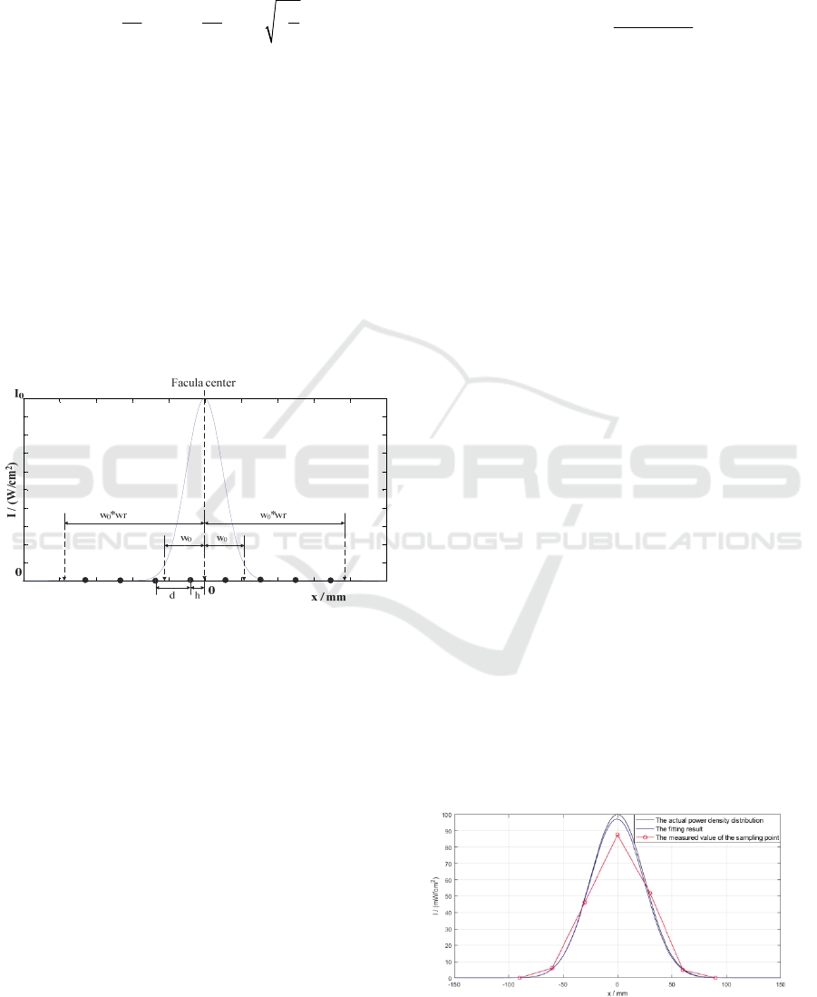
The position of the sampling point on the actual

detector array is given, and the facula wobbles within

a certain range. For the convenience of calculation, it

is assumed that the facula is fixed, and sampling points

are set uniformly. In this way, three parameters are

involved in the distribution of sampling points, as

shown in Figure 1. They are d, wr, and h, which stand

for the interval of sampling points, the ratio of

sampling point range to facula diameter, and the

distance between the facula center and the sampling

point on the left side of it. Parameters of d and wr are

related to the design of detector array. Parameter of h

changes randomly in the actual measurement, with the

range of 0~d/2.

Figure 1: Physical meaning of parameters in simulation

calculation.

For each set of d, wr and h, the coordinates x

of each

sampling point can be determined. Then the true value

I(x

) of each sampling point can be obtained by

substituting x

to formula (1). There is a certain

measurement error for each sampling points, which

follows the normal distribution with the mean value of

0 and the standard deviation of δ

. A group of random

error values δ

(i=1, 2, … , n, n is the number of

sampling points) that meet the above normal

distribution are selected, so the measured value of each

sampling point is I'(x

)= I(x

)*(1+δ

). Substituting it

into formula (2), z'(x

)=ln(I'(x

)) is obtained. In

MATLAB, the least square fitting of (x

，z'(x

)) is

carried out using the polyfit function (Shenyong Ruan,

Yongli Wang, Qunfang Sang, 2004), and three

coefficients of a

, b

and c

are obtained. Then, the

fitting coefficients x

, w

and I

are calculated

according to formula (3). Here, the subscript "1"

represents the fitting result.

Therefore, the power density distribution function

obtained by fitting is:

()

101

() exp

Ix I



−

=⋅ −





(4)

Compared with the true value in formula (1), the fitting

error values of facula center (x

-x

), facula radius

-w

), and center power density (I

-I

) are obtained.

A number of m groups of random error are selected,

and a group of fitting error, such as (x

-x

)

, (w

-w

)

and (I

-I

)

, j = 1, 2, ... , m, is obtained for each group

of random error according to the above process. Then

the fitting error under the conditions of d, wr and h is

acquired by the standard deviation of m groups of

fitting error values is calculated.

2.2 Initial Conditions of

One-dimensional Simulation

The initial conditions used in the calculation are:

1) The facula center x

=0. The facula radius w

=50mm.

The center power density I

=100mW/cm

2) The ratio of the sampling point range to the facula

diameter wr=2. The sampling point interval d is

changed from 30mm to 60mm, and the step is 1mm.

The distance between the facula center and the

sampling point on the left side of it h is changed from

0 to d/2, and the step is d/8.

3) the standard deviation of sampling point error is

=15%.

4) The number of groups of random error m = 10000.

2.3 Results of One-dimensional

Simulation

When d=30mm, wr=2, h=0mm, a group of random

error of sampling points is selected, and the fitting

result for the measured values of sampling points is as

Figure 2:

Figure 2: Result of one-dimensional fitting.

Inﬂuence of Sampling Point Setting on Fitting Error of Ideal Gaussian Beam

141

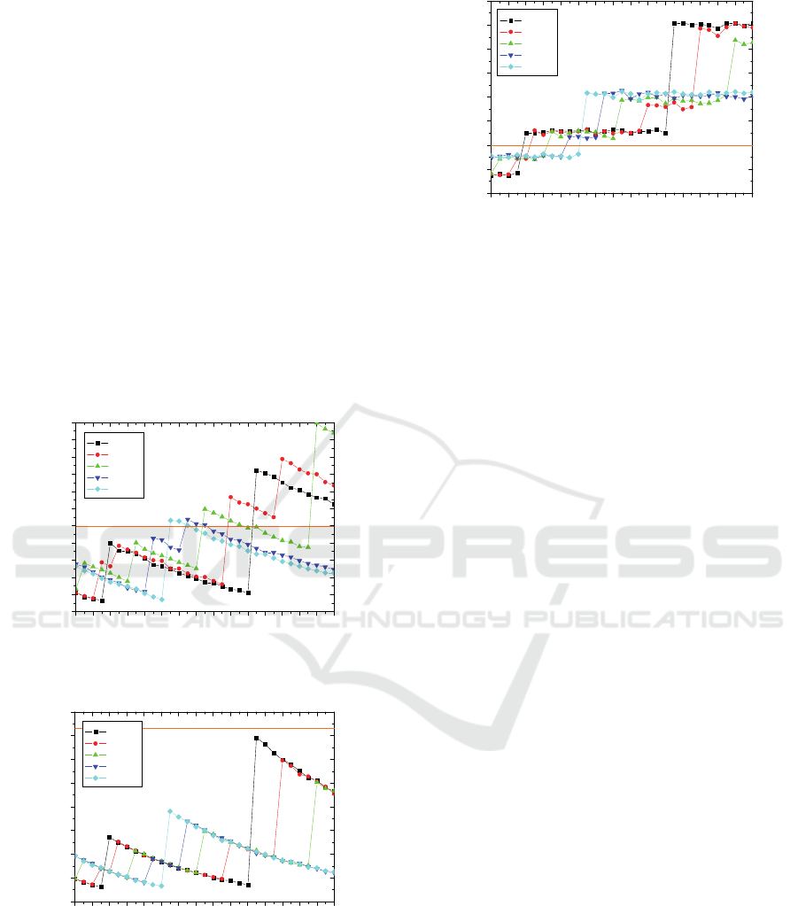
In the figure, the black line represents the actual power

density distribution, the red circle represents the

measured value of the sampling point, and the blue line

represents the power density distribution obtained by

fitting the measured value of the sampling points,

where x

=0.46mm, w

=49.80mm and

=97.18mW/cm

, and the fitting errors are (x

)=0.46mm, (w

-w

)=-0.20mm, and (I

-I

)=-

2.82mW/cm

A number of m=10000 groups of random error

values are selected, and a number of m=10000 groups

of the fitting error is obtained. Then the fitting error

under the conditions of d=30mm, wr=2 and h=0mm is

obtained: the fitting error of the facula center is

=0.61mm, the fitting error of the facula radius is

=0.59mm, and the fitting error of the center power

density is δ

=8.73mW/cm

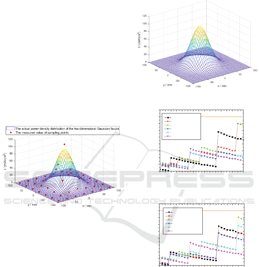
When d and h change in the calculation range, the

simulation results of the fitting errors are as shown in

Figure 3 ~ Figure 5.

Figure 3: Fitting error of the facula center for one-

dimensional simulation.

Figure 4: Fitting error of the facula radius for one-

dimensional simulation.

It can be seen from the figure:

1) The relationship between fitting error and sampling

interval is not monotonous increasing or decreasing,

but segmented. With the increase of d, the overall

errors of the next section is higher than that of the

Figure 5: Fitting error of the center power density for one-

dimensional simulation.

previous section. While in a certain section, it is

basically monotonic decreasing. This is because in a

certain

range, the number of sampling points is

constant. The larger d is, the wider the distribution of

sampling points is, the more information is detected,

and the smaller the fitting error is. When d increases to

a certain value, because wr is limited to 2, the number

of sampling points decreases, so the detection

information decreases, and the fitting error suddenly

increases. Taking h=0 as an example, the range of

sampling points is limited to w

*wr=50*2=100mm.

When d=30-33mm, there are three sampling points on

both sides of the facula center. When d=34-50mm,

there are two sampling points on both sides of the

facula center. When d=51-60mm, there is one

sampling point on both sides of the facula center.

Therefore, the boundary between segments are

between d=33mm and d=34mm, d=50mm and

d=51mm.

2) It is assumed that, the admissible errors of the facula

center, facula radius and center power density are 1mm,

2.5mm (5%) and 10mW/cm

(10%), respectively,

which are represented by solid red lines in the figures.

When selecting the interval of sampling points d, the

fitting errors should not exceed the admissible ones

under all h conditions. It can be seen from the figures

that, within the initial condition range of simulation

calculation, the fitting error of facula radius is smaller

than the admissible one, and the fitting errors of facula

center and center power density do not exceed the

admissible ones when d ≤ 40mm and d ≤ 33mm

respectively. Therefore, d≤33mm should be selected

to ensure the fitting accuracy.

30 32 34 36 38 40 42 44 46 48 50 52 54 56 58 6

0.5

0.6

0.7

0.8

0.9

1.0

1.1

1.2

1.3

1.4

1.5

1.6

error of x

/ mm

d / mm

h/d=0

h/d=1/8

h/d=1/4

h/d=3/8

h/d=1/2

30 32 34 36 38 40 42 44 46 48 50 52 54 56 58 60

0.3

0.6

0.9

1.2

1.5

1.8

2.1

2.4

2.7

h/d=0

h/d=1/8

h/d=1/4

h/d=3/8

h/d=1/2

error of w

/ mm

d / mm

30 32 34 36 38 40 42 44 46 48 50 52 54 56 58 60

h/d=0

h/d=1/8

h/d=1/4

h/d=3/8

h/d=1/2

error of I

/ (mW/cm

)

d / mm

PHOTOPTICS 2020 - 8th International Conference on Photonics, Optics and Laser Technology

142

3 TWO-DIMENSIONAL

SIMULATION

3.1 Calculation Method of

Two-dimensional Simulation

The general expression of the power density

distribution function of the two-dimensional Gaussian

beam cross-section facula is as follows:

()()

(, ) exp

xx yy

Ixy I



−−

=⋅ − −





(5)

Where (x

, y

) is the facula center, (w

, w

) is the

facula radius in the X and Y directions, and I

is the

center power density.

Similar to the one-dimensional simulation

calculation, equation (5) is transformed by logarithm

operation on both sides of the equal sign.

ln ( , ) ,

z I x y ax bx cy dy e c





=−



==++++=−





=−−





(6)

The coefficients a, b, c, d and e can be obtained by the

second order polynomial fitting of the transformed

function. According to the relationship between the

transformed function and the original Gaussian

function, the corresponding parameters of the Gaussian

function can be obtained as follow:

000

exp , ,

44 2

bd b

Ie x

ac a

wyw

ac c



=−− =−





=− =− =−

(7)

Similar to the one-dimensional simulation calculation

shown in Figure 1, four parameters are involved in the

two-dimensional distribution of sampling points.They

are the interval of sampling points d, the ratio of

sampling point range to facula diameter wr, the

distance between the facula center and the sampling

point on the left side of it hx, and the distance between

the facula center and the sampling point under it

hy.Parameters of d and wr are related to the design of

detector array. Parameters of hx and hy change

randomly in the actual measurement, with the range of

0~d/2.

For each set of d, wr, hx and hy, the coordinates (x

) of each sampling point can be determined, where

i=1, 2,... , nx, j=1, 2,... , ny, nx and ny represent the

number of columns and rows of sampling points

respectively. The true value I(x

, y

) of each sampling

point is obtained by substituting (x

, y

) to formula (5).

A group of random error values δ

are selected, and the

measured value of each sampling point is I'(x

, y

)= I(x

)*(1+δ

). Substituting it into formula (6), z'(x

)=ln(I'(x

, y

)) is obtained. Then the least square fitting

of ((x

， y

) ， z'(x

, y

)) is carried out, and five

coefficients of a

, b

, c

, d

and e

are obtained. So, the

fitting coefficients (x

, y

), (w

0x1

, w

0y1

) and I

are

calculated according to formula (7).

So far, the power density distribution function of

the two-dimensional Gaussian beam cross-section

facula is obtained by fitting:

()()

01 01

101

01 01

(, ) exp

xx yy

Ixy I





−−

=⋅ − −













(8)

Compared with the true value in formula (5), the fitting

errors of facula center (x

-x

, y

-y

), facula radius

0x1

-w

, w

0y1

-w

), and center power density (I

-I

)

are obtained.

A number of m groups of random error are selected,

and a group of fitting error, such as (x

-x

, y

-y

)

0x1

-w

, w

0y1

-w

)

and (I

-I

)

, j = 1, 2, ... , m, is

obtained for each group of random error according to

the above process. Then The fitting error under the

conditions of d, wr hx and hy is acquired by the

standard deviation of m groups of fitting error values is

calculated.

3.2 Initial Conditions of

Two-dimensional Simulation

The initial conditions used in the calculation are:

1) The facula center (x

)=(0,0). The facula radius

=50mm. The center power density

=100mW/cm

2) The ratio of the sampling point range to the facula

diameter wr=2. The sampling point interval d is

changed from 30mm to 60mm, and the step is 1mm.

The distance between the facula center and the

sampling point on the left side of it hx is changed from

0 to d/2, and the step is d/4. The distance between the

facula center and the sampling point under it hy is

changed from 0 to hx, and the step is d/4.

3) the standard deviation of sampling point error is

=15%.

Inﬂuence of Sampling Point Setting on Fitting Error of Ideal Gaussian Beam

143

4) The number of groups of random error m = 10000.

3.3 Results of Two-dimensional

Simulation

The actual distribution of the power density of the two-

dimensional Gaussian facula is shown in Figure 6.

When d=30mm, wr=2, hx=hy=0mm, a group of

random error of sampling points is selected, and the

measured value of sampling points is obtain as shown

in the red dot in Figure 6. The power density

distribution obtained by fitting the measured value of

the sampling points is shown in Figure 7, where

=0.30mm, w

0x1

=49.82mm, y

=0.32mm,

0y1

=49.98mm and I

=101.00mW/cm

, and the fitting

errors are (x

-x

)=0.30mm, (w

0x1

-w

)=-0.18mm, (y

)=0.32mm, (w

0y1

-w

)=-0.02mm and (I

)=1.00mW/cm

, respectively.

Figure 6: Gaussian facula and measured value of sampling

points.

A number of m=10000 groups of random error values

are selected, and a number of m=10000 groups of the

fitting errors (x

-x

)

, (w

0x1

-w

)

, (y

-y

)

, (w

0y1

-w

)

and (I

-I

)

are obtained. Then the fitting errors under

the conditions of d=30mm, wr=2 and hx=hy=0mm are

obtained: the fitting error of the facula center is (δ

)=(0.23mm, 0.23mm), the fitting error of the facula

radius is (δ

w0x

, δ

w0y

)=(0.22mm, 0.22mm), and the

fitting error of the center power density is

=4.16mW/cm

When d, hx and hy change in the calculation range,

the simulation results of the fitting errors are as shown

in Figure 8 ~ Figure 12.

It can be seen from the above data:

1) Within the range of initial conditions of simulation

calculation, the fitting error of two-dimensional

simulation is less than that of one-dimensional

simulation. The reason is: there are more sampling

points

distributed in two-dimensional, and more

Figure 7: Result of two-dimensional fitting.

Figure 8: Fitting error of the facula center x

for two-

dimensional simulation.

Figure 9: Fitting error of the facula center y

for two-

dimensional simulation.

information is detected, then the fitting error is smaller.

2) The relationship between the fitting error and the

interval of sampling points is not monotonous

increasing or decreasing, but segmented. Because the

number of sensors has changed. With the increase of d,

the overall error of the next section is higher than that

of the previous section. While in a certain section, it is

basically monotonic decreasing. This is consistent with

one-dimensional simulation.

30 32 34 36 38 40 42 44 46 48 50 52 54 56 58 60

0.2

0.3

0.4

0.5

0.6

0.7

0.8

0.9

1.0

1.1

hx/d=0 hy/d=0

hx/d=1/4 hy/d=0

hx/d=1/4 hy/d=1/4

hx/d=1/2 hy/d=0

hx/d=1/2 hy/d=1/4

hx/d=1/2 hy/d=1/2

error of x

/ mm

d / mm

30 32 34 36 38 40 42 44 46 48 50 52 54 56 58 60

0.2

0.3

0.4

0.5

0.6

0.7

0.8

0.9

1.0

1.1

hx/d=0 hy/d=0

hx/d=1/4 hy/d=0

hx/d=1/4 hy/d=1/4

hx/d=1/2 hy/d=0

hx/d=1/2 hy/d=1/4

hx/d=1/2 hy/d=1/2

error of y

/ mm

d / mm

PHOTOPTICS 2020 - 8th International Conference on Photonics, Optics and Laser Technology

144

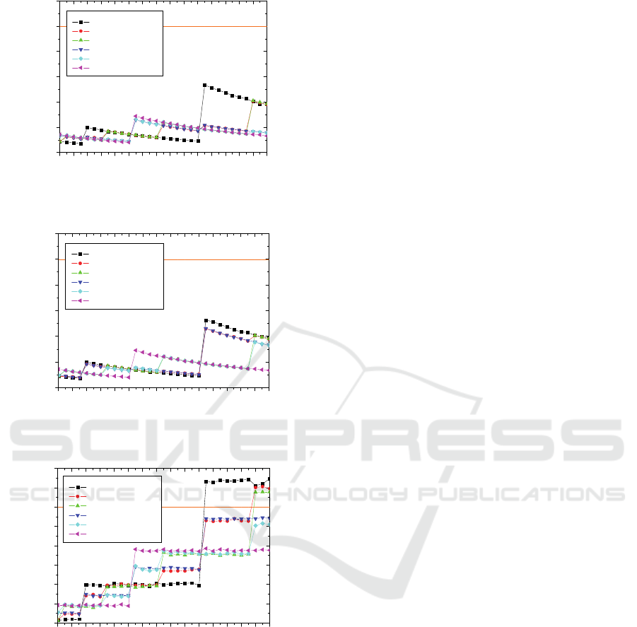
Figure 10: Fitting error of the facula radius w

for two-

dimensional simulation.

Figure 11: Fitting error of the facula radius w

for two-

dimensional simulation.

Figure 12: Fitting error of the center power density for two-

dimensional simulation.

3) It is assumed that, the admissible errors of the facula

center, facula radius and center power density are

1mm, 2.5mm (5%) and 10mW/cm

(10%),

respectively, which are represented by solid red lines

in the figure. When selecting the interval of sampling

points d, the fitting errors should not exceed the

admissible ones under all hx and hy conditions. It can

be seen from the figure that, in the initial condition

range of the simulation calculation, the fitting errors of

the facula center and the facula radius are smaller than

the admissible ones, and the fitting error of the center

power density exceeds the admissible one when

d>50mm. Therefore, in the design, d≤50mm should

be selected to ensure that all fitting errors do not exceed

the admissible ones. The interval range of sampling

points is larger than that allowed by one-dimensional

simulation.

4 CONCLUSIONS

Based on MATLAB and least square method, the one-

dimensional and two-dimensional fitting of Gaussian

distribution facula are carried out. The influence of

sampling point layout on fitting error is studied, and the

relationship between the fitting error and sampling

point interval is analyzed. The results show that, the

number of sampling points in the two-dimensional

simulation is larger, and the fitting accuracy is better

than that in the one-dimensional simulation under the

same sampling point interval. Because the actual facula

is a two-dimensional Gaussian distribution, the two-

dimensional simulation results shall be prioritized.

In the range of initial conditions of simulation

calculation, the interval of sampling points should be d

≤50mm, so that the fitting errors of facula center,

facula radius and center power density can be

controlled within the admissible ones.

REFERENCES

Bingkun Zhou, Yizhi Gao, Tirong Chen, et al.. 2000. Laser

principle(4th edition), National Denfense Industry Press,

Beijing.

Shenyong Ruan, Yongli Wang, Qunfang Sang, 2004.

MATLAB program design, Publishing house of

electronics industry, Beijing.

Lili Wang, Zhongwen Hu, Hangxin Ji, 2012. Laser facula

center location algorithm based on Gaussian fitting,

Journal of Applied Optics, 33(5), 985.

Bing Kong, Zhao Wang, Yusan Tan, 2002. Gaussian fitting

technique of laser facula, Laser Technology, 26(4),277.

C. Higgs, P.C. Grey, J.G. Mooney. 1999. Dynamic target

board for ABL ACT performance characterization,

Proceeding of SPIE, 3706, 216

J. Thomas Knudtson, Kenneth L. Ratzlaff. 1983. Laser beam

spatial profile analysis using a two-dimensional

photodiode array, Rev.Sci.Instrum, 54(7),856

30 32 34 36 38 40 42 44 46 48 50 52 54 56 58 60

0.0

0.5

1.0

1.5

2.0

2.5

3.0

hx/d=0 hy/d=0

hx/d=1/4 hy/d=0

hx/d=1/4 hy/d=1/4

hx/d=1/2 hy/d=0

hx/d=1/2 hy/d=1/4

hx/d=1/2 hy/d=1/2

error of w

/ mm

d / mm

30 32 34 36 38 40 42 44 46 48 50 52 54 56 58 6

0.0

0.5

1.0

1.5

2.0

2.5

3.0

hx/d=0 hy/d=0

hx/d=1/4 hy/d=0

hx/d=1/4 hy/d=1/4

hx/d=1/2 hy/d=0

hx/d=1/2 hy/d=1/4

hx/d=1/2 hy/d=1/2

error of w

/ mm

d / mm

30 32 34 36 38 40 42 44 46 48 50 52 54 56 58 60

error of I

/ (mW/cm

)

d / mm

hx/d=0 hy/d=0

hx/d=1/4 hy/d=0

hx/d=1/4 hy/d=1/4

hx/d=1/2 hy/d=0

hx/d=1/2 hy/d=1/4

hx/d=1/2 hy/d=1/2

Inﬂuence of Sampling Point Setting on Fitting Error of Ideal Gaussian Beam

145