Interactive Axis-based 3D Rotation Speciﬁcation using Image Skeletons

Xiaorui Zhai

1 a

, Xingyu Chen

1,2 b

, Lingyun Yu

1 c

and Alexandru Telea

3 d

Bernoulli Institute, University of Groningen, The Netherlands

School of Computer and Communication Engineering, University of Science and Technology, Beijing, China

Utrecht University, The Netherlands

Keywords:

Skeletonization, 3D Interaction, Image-based Techniques.

Abstract:

Specifying 3D rotations of shapes around arbitrary axes is not easy to do. We present a new method for this

task, based on the concept of natural local rotation axes. We deﬁne such axes using the 3D curve skeleton

of the shape of interest. We compute effective and efﬁcient approximations of such skeletons using the 2D

projection of the shape. Our method allows users to specify 3D rotations around parts of arbitrary 3D shapes

with a single click or touch, is simple to implement, works in real time for large scenes, can be easily added to

any OpenGL-based scene viewer, and can be used on both mouse-based and touch interfaces.

1 INTRODUCTION

Interactive manipulation of 3D scenes is a key part

of many applications such as CAD/CAM modeling,

computer games, and scientiﬁc visualization (Jackson

et al., 2013). 3D rotations are an important manip-

ulation type, as they allow examining scenes from

various viewpoints to e.g. select the most suitable one

for the task at hand. Two main 3D rotation types ex-

ist – rotation around a center and rotation around an

axis. The ﬁrst one can be easily speciﬁed via classi-

cal (mouse-and-keyboard) (Zhao et al., 2011) or touch

interfaces (Yu et al., 2010) by well-known metaphors

such as the trackball. The latter is also easy to specify

if the rotation axis coincides with one of the world-

coordinate axes. Rotations around arbitrary axes are

considerably harder to specify, as this requires a total

of 7 degrees of freedom (6 for specifying the axis and

one for the rotation angle around the axis).

Users often do not need to rotate around any 3D

axis. Consider the case when one wants to examine

a (complex) 3D shape such as a statue: It can be ar-

gued that a good viewpoint will display the statue in a

‘natural’ position, i. e., with the head upwards. Next, a

‘natural’ way to rotate this shape is around its vertical

symmetry axis. This keeps the shape’s global orienta-

https://orcid.org/0000-0002-4244-9485

https://orcid.org/0000-0002-3770-4357

https://orcid.org/0000-0002-3152-2587

https://orcid.org/0000-0003-0750-0502

tion (which helps understanding the shape) but allows

one to examine it from all viewpoints.

Several methods support the above exploration

scenario by ﬁrst aligning a shape’s main symmetry

axis with one of the world coordinate axes and then

using a simple-to-specify rotation around this world

axis (Dufﬁn and Barrett, 1994). This scenario falls

short when (a) the studied shape does not admit a

global symmetry axis, although its parts may have

local symmetry axes; (b) computing such (local or

global) symmetry axes is not simple; or (c) we do not

want to rotate along an axis which is ﬁrst aligned with

a world axis.

To address the above, we propose a novel inter-

action mechanism: Given a shape viewed from an

arbitrary 3D viewpoint, we allow the user to choose a

part of interest of the shape. Next, we propose a fast

and generic method to compute an approximate 3D

symmetry axis for this part. Finally, we interactively

rotate the shape around this axis by the desired angle.

This effectively allows one to rotate the viewpoint to

examine shapes around a multitude of symmetry axes

that they can easily select. Our method can handle any

3D shape or scene, e.g., polygon mesh or polygon soup,

point-based or splat-based rendering, or combination

thereof; is simple to implement and works at interac-

tive rates even for scenes of hundreds of thousands

of primitives; requires no preprocessing of the 3D ge-

ometry; and, most importantly, allows specifying the

rotation axis and rotation angle by a single click, there-

fore being suitable for both classical (mouse-based)

Zhai, X., Chen, X., Yu, L. and Telea, A.

Interactive Axis-based 3D Rotation Speciﬁcation using Image Skeletons.

DOI: 10.5220/0009149901690178

In Proceedings of the 15th International Joint Conference on Computer Vision, Imaging and Computer Graphics Theory and Applications (VISIGRAPP 2020) - Volume 1: GRAPP, pages

169-178

ISBN: 978-989-758-402-2; ISSN: 2184-4321

169

and touch interfaces. We demonstrate our method on

several types of 3D scenes and exploration scenarios.

2 RELATED WORK

Rotation Speciﬁcation.

Many mechanisms for

specifying 3D scene rotation exist. The trackball

metaphor (Bade et al., 2005; Zhao et al., 2011) is one

of the oldest and likely most frequently used. Given a

3D center-of-rotation

, the scene is rotated around an

axis passing through

and determined by the projec-

tions on a hemisphere centered at

of the 2D screen-

space locations

and

corresponding to a mouse

pointer motion. The rotation angle

is controlled

by the amount of pointer motion. Trackball rotation

is simple to implement and allows freely rotating a

shape to examine it from all viewpoints. Yet, control-

ling the actual axis around which one rotates is hard,

as this axis constantly changes while the user moves

the mouse. At the other extreme, world-coordinate-

axis rotations allow rotating a 3D scene around the

, or

axes (Zhao et al., 2011; Jackson et al., 2013).

The rotation axis and rotation amount

can be cho-

sen by simple click-and-drag gestures in the viewport.

This method works best when the scene is already pre-

aligned with a world axis, so that rotating around that

axis provides meaningful viewpoints.

Pre-alignment of 3D models is a common prepro-

cessing stage in visualization (Chaouch and Verroust-

Blondet, 2009). Principal Component Analysis (PCA)

does this by computing a shape’s eigenvectors

and

, ordered by the respective eigenvalues

≥

≥ λ

, so that the coordinate system

}

is right-

handed. Next, the shape can be suitably aligned with

the viewing coordinate system

by a simple

3D rotation around the shape’s barycenter (Tangelder

and Veltkamp, 2008; Kaye and Ivrissimtzis, 2015).

3D rotations can be speciﬁed by classical (mouse-

and-keyboard) (Zhao et al., 2011) but also touch inter-

faces. Yu et al. (Yu et al., 2010) presented a direct-

touch exploration technique for 3D scenes called

Frame Interaction with 3D space (FI3D). Guo et

al. (Guo et al., 2017) extended FI3D with constrained

rotation, trackball rotation, and rotation around a user-

deﬁned center. (Yu and Isenberg, 2009) used trackball

interaction to control rotation around two world axes

by mapping it to single-touch interaction.

Medial Descriptors.

Medial descriptors, also

known as skeletons, are used for decades to capture

the symmetry structure of shapes (Siddiqi and Pizer,

2008). For shapes

Ω ⊂ R

n ∈ {2, 3}

with boundary

∂ Ω, skeletons are deﬁned as

Ω

={x ∈ Ω|∃f

∈ ∂ Ω,f

∈ ∂ Ω : f

6= f

∧

||x −f

|| = ||x − f

|| = DT

Ω

(x)} (1)

where

are called the feature points of skeletal point

and

Ω

is the distance transform (Rosenfeld and

Pfaltz, 1968) of skeletal point x, deﬁned as

Ω

(x ∈ Ω) = min

y∈∂ Ω

kx −yk. (2)

The feature points deﬁne the so-called feature trans-

form (Hesselink and Roerdink, 2008)

Ω

(x ∈ Ω) = argmin

y∈∂ Ω

kx −yk. (3)

In 3D, two skeleton types exist (Tagliasacchi et al.,

2016): Surface skeletons, deﬁned by Eqn 1 for

Ω ⊂ R

consist of complex intersecting manifolds with bound-

ary, and hence are hard to compute and utilize. Curve

skeletons are curve-sets in

that locally capture the

tubular symmetry of shapes. They are structurally

much simpler than surface skeletons and enable many

applications such as shape segmentation (Rodrigues

et al., 2018) and animation (Bian et al., 2018). Yet,

they still cannot be computed in real time, and require

a well-cured deﬁnition of

Ω

as either a watertight, non-

self-intersecting, ﬁne mesh (Sobiecki et al., 2013), or

a high-resolution voxel volume (Reniers et al., 2008).

3 PROPOSED METHOD

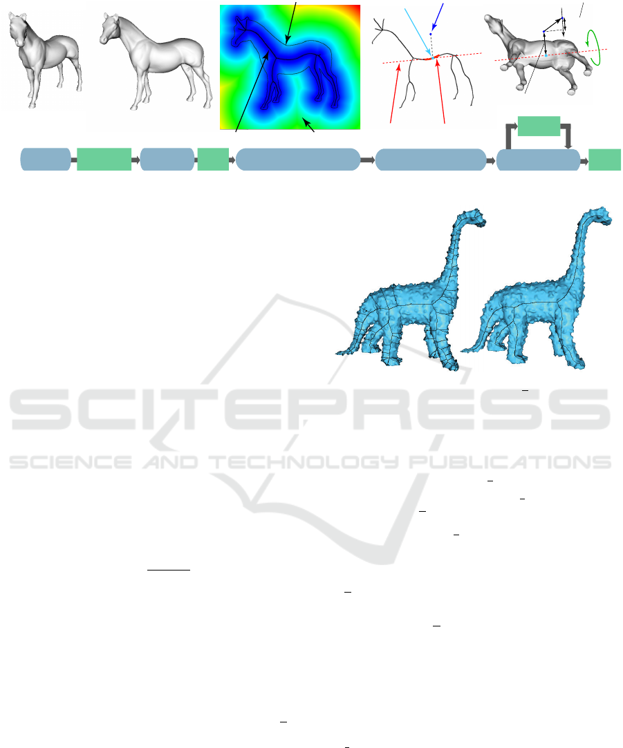
We construct a 3D rotation in ﬁve steps (Fig. 1) which

can be integrated into any OpenGL-based 3D scene

viewer. We start by loading the scene of interest into

the viewer (a). Next, the user can employ any standard

mechanisms offered by the viewer, e.g. trackball rota-

tion, zoom, or pan, to choose a viewpoint of interest,

from which the viewed scene shows a detail around

which one would like to further rotate to explore the

scene. In our example, such a viewpoint (b) shows the

horse’s rump, around which we next want to rotate the

horse to view it from different angles.

3.1 Rotation Axis Computation

From the above-mentioned initial viewpoint, we next

perform three image-space operations to compute the

3D rotation axis. These steps, denoted A, B, and C

next, are as follows.

A. Silhouette Extraction.

This is the ﬁrst operation

in step (d) in Fig. 1. We render the shape with Z

buffering on and using the standard

GL LESS

OpenGL

GRAPP 2020 - 15th International Conference on Computer Graphics Theory and Applications

170

click

to start

e) rotation axis estimation

sihouette boundary ∂Ω

skeleton S

distance field DT

clicked point p

skeleton

anchor s

skeleton

neighbors N(s

)

rotation

axis a

||p-s

|| = rotation speed

(single click mode)

b) free

manipulation

c) viewpoint

of interest

d) image-space computations

(silhouette, skeleton, Z-buffers)

f) rotation along

local axis

move

to control

release

to end

a) initial

pose

n×a

d (n×a)

rotation angle

(click & drag mode)

Figure 1: Skeleton-based local rotation pipeline. Blue boxes indicate tool states. Green boxes indicates user actions.

depth-test. Let

Ω

near

be the resulting Z buffer. We next

ﬁnd the silhouette

Ω

of the rendered shape as all pixels

that have a value in

Ω

near

different from the default

(the latter being 1 for standard OpenGL settings).

B. Skeleton Computation.

We next compute the sil-

houette skeleton

Ω

following Eqn. 1. This is the

second operation in step (d) in Fig. 1. To eliminate

spurious skeletal branches caused by small-scale noise

along

∂ Ω

, we regularize

Ω

by using the salience-

based metric in (Telea, 2011). Brieﬂy put, this regular-

ization works as follows. For every point

x ∈ S

Ω

of the

full skeleton computed by Eqn. 1, we compute ﬁrst the

so-called importance

ρ(x) ∈ R

, deﬁned as the short-

est path along

∂ Ω

between the two feature points

and

. As shown in (Telea and van Wijk, 2002),

monotonically increases along skeletal branches from

their endpoints to the skeleton center, and equals, for a

skeleton point

, the amount of boundary length which

is captured (described) by

. Next, the saliency of

point x is deﬁned as

σ(x) =

ρ(x)

Ω

(x)

. (4)

As shown in (Telea, 2011), the saliency is overall

low on skeleton branches caused by small-scale de-

tails along

∂ Ω

and overall high on skeleton branches

caused by important (salient) protrusions of

∂ Ω

Hence, we can regularize

Ω

simply by removing all

its pixels having a salience value lower than a ﬁxed

threshold

. Following (Telea, 2011), we set

= 1

Figure 2 illustrates the regularization process by show-

ing the raw skeleton

Ω

and its regularized version

Ω

for a noisy shape. As visible in image (b), the salience

regularization removes all spurious branches created

by surface noise, but leaves the main skeleton branches,

corresponding to the animal’s limbs, rump, and tail,

intact. Salience regularization is simple and automatic

to use, requiring no parameters to be controlled by the

user – for details, we refer to (Telea, 2011).

a) noisy (non-regularized)

skeleton S

b) regularized

skeleton S

Figure 2: Raw skeleton

Ω

with noise-induced branches (a)

and saliency-based regularized version S

Ω

(b).

C. Rotation Axis Computation.

This is step (e) in

Fig. 1. Let

be the pixel under the user-manipulated

pointer (blue in Fig. 1e). We ﬁrst ﬁnd the closest

skeleton point s

= argmin

y∈S

Ω

kp −yk by evaluating

the feature transform (Eqn. 3)

Ω

(p)

of the regu-

larized skeleton

Ω

. Figure 1d shows the related

distance transform

Ω

. In our case,

is a point

on the horse’s rump skeleton (cyan in Fig. 1e). Next,

we ﬁnd the neighbor points

N(s

)

by searching

depth-ﬁrst from

along the pixel connectivity-graph

Ω

up to a maximal distance set to

10%

of the

viewport size.

N(s

)

contains skeletal points along

a single branch in

Ω

, or a few connected branches,

is close to a skeleton junction. In our case,

N(s

)

contains a fragment of the horse’s rump skele-

ton (red in Fig. 1e). For each

q ∈ N(s

)

, we next

estimate the depth

as the average of

Ω

f ar

(q)

and

Ω

near

(q)

. Here,

Ω

f ar

is the Z buffer of the scene

rendered with front-face culling on and the standard

GL LESS

OpenGL depth-test, giving thus the depth of

the nearest backfacing-polygons to the view plane.

Figure 3 illustrates this. First (a), the user clicks

above the horse’s rump and drags the pointer upwards.

Image (b) shows the resulting rotation. As visible,

the rotation axis (red) is centered inside the rump, as

its depth

is the average of the near and far rump

Interactive Axis-based 3D Rotation Speciﬁcation using Image Skeletons

171

faces. Next (c), we consider a case of overlapping

shape parts. The user clicks left to the horse’s left-

front leg, which overlaps the right-front one. Image

(d) shows the resulting rotation. Again, the rotation

axis (red) is centered inside the left-front leg. In this

case,

Ω

f ar

(q)

contains the Z value on the backfacing

part of the left-front leg, so

(Ω

near

(q) + Ω

f ar

(q))/2

yields a value roughly halfway this leg along the Z

axis. Separately, we handle non-watertight surfaces as

follows: If

Ω

f ar

(q)

contains the default (maximal) Z

value, this means there’s no backfacing surface under

a given pixel

, so the scene is not watertight at that

point. We then set q

to Ω

near

(q).

a) b)

c) d)

clicked

point p

clicked

point p

rotation

Figure 3: Depth estimation of rotation axis for (a,b) non-

overlapping part and (c,d) overlapping parts. In both cases,

the rotation axis (red) is nicely centered in the shape.

We now have a set

= {(q ∈ N(s

),q

)}

of 3D

points that approximate the 3D curve skeleton of our

shape close to the pointer location

. We set the 3D

rotation axis

to the line passing through the average

point of

and oriented along the largest eigenvector

of N

’s covariance matrix (Fig. 1e, red dotted line).

3.2 Controlling the Rotation

We offer three interactive mechanisms to control the

rotation (step (f) in Fig. 1), as follows.

Indication.

As the user moves the pointer

, we con-

tinuously update the display of

. This shows along

which axis the scene would rotate if the user initiated

the rotation from

. If

is found suitable, one can start

rotating by a click following one of the two modes

listed next; else one can move the pointer

to ﬁnd a

more suitable axis;

Single Click.

In this mode, we compute a rotation

speed

equal to the distance

kp −s

and a rotation

direction

(clockwise or anticlockwise) given by the

sign of the cross-product

− p)× n

, where

is the

viewplane normal. We next continuously rotate (spin)

the shape around a with the speed σ in direction δ ;

Click and Drag.

Let

be the drag vector created by

the user as she moves the pointer

from the current

to the next place in the viewport with the control, e.g.

mouse button, pressed. We rotate the scene around

with an angle equal to d ·(n ×a) (Fig. 1e).

We stop rotation when the user release the control

(mouse button, touchpad, or touch screen). In single-

click mode, clicking closer to the shape rotates slowly,

allowing to examine the shape in detail. Clicking far-

ther rotates quicker to e.g. explore the shape from the

opposite side. The rotation direction is given by the

side of the skeleton where we click: To change from

clockwise to counterclockwise rotation in the example

in Fig. 1, we only need to click below, rather than

above, the horse’s rump. In click-and-drag mode, the

rotation speed and direction is given by the drag vector

: Values

orthogonal to the rotation axis

create

corresponding rotations clockwise or anticlockwise

around

; values

along

yield no rotation. This

matches the intuition that, to rotate along an axis, we

need to move the pointer across that axis.

a) b)

c) d)

wrong skeleton

branches

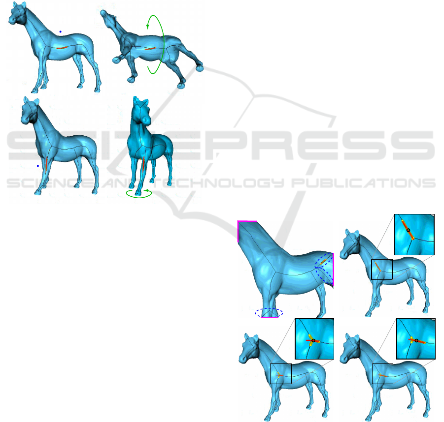
Figure 4: Two problems of estimating rotation axes from

skeletons. (a) Zoomed-in scene. (b-d) Anchor points close

to a skeleton junction. See Sec. 3.3.

GRAPP 2020 - 15th International Conference on Computer Graphics Theory and Applications

172

The skeleton-based construction of the rotation axis is

key to the effectiveness of our approach: If the shape

exhibits some elongated structure in the current view

(e.g. rump or legs in Fig. 1c), this structure will yield a

skeleton branch. Clicking closer to this structure than

to other structures in the same view – e.g., clicking

closer to the rump than to the horse’s legs or neck –

selects the respective skeleton branch to rotate around.

This way, the 3D rotation uses the ‘natural’ structure

of the viewed shape. We argue that this makes sense

in an exploratory scenario, since, during rotation, the

shape parts we rotate around stay ﬁxed in the view, as

if one ‘turns around’ them.

The entire method requires a single click and, op-

tionally, a pointer drag motion to execute. This makes

our method simpler than other 3D rotation methods

that rotate around freely speciﬁable 3D axes, and also

directly applicable to contexts where no second but-

ton or modiﬁer keys are available, e.g., touch screens.

Moreover, our method does not require any complex

(and/or slow) 3D curve-skeleton computation: We

compute only 2D (silhouette) skeletons, which are

fast and robust to extract (Telea and van Wijk, 2002;

Ersoy et al., 2011). We can handle any 3D input ge-

ometry, e.g., meshes, polygon soups, point clouds, or

mixes thereof, as long as such primitives render in the

Z buffer (see Sec. 4 for examples hereof).

3.3 Improvements of Basic Method

We next present three improvements of the basic local-

axis rotation mechanism described above.

Zoom Level.

A ﬁrst issue regards computing the

scene’s 2D silhouette

Ω

(Sec. 3.1A). For this to work

correctly, the entire scene must be visible in the cur-

rent viewport. If this is not the case, the silhouette

boundary

∂ Ω

will contain parts of the viewport bor-

ders. Figure 4a shows this for a zoomed-in view of the

horse model, with the above-mentioned border parts

marked purple. This leads to branches in the skeleton

Ω

that do not provide meaningful rotation axes. We

prevent this to occur by requiring that the entire scene

is visible in the viewport before initiating the rotation-

axis computation. If this is not the case, we do not

allow the skeleton-based rotation to proceed, but map

the user’s interaction to a traditional trackball-based

rotation.

Skeleton Junctions.

If the user selects

so that the

skeleton anchor

is too close to a skeleton junction,

then the neighbor-set

N(s

)

will contain points belong-

ing to more than two branches. Estimating a line from

such a point set (Sec. 3.1C) is unreliable, leading to

possibly meaningless rotation axes. Figures 4b-d illus-

trates the problem. The corresponding skeleton points

N(s

)

used to estimate the axis are shown in yellow,

and the resulting axes in red. When

is relatively far

from the junction (Figs. 4b,d),

N(s

)

contains mainly

points from a single skeleton branch, so the estimated

rotation axes are reliable. However, when

is very

close to the junction (Fig. 4c),

N(s

)

contains points

from all three meeting branches, so, as the user moves

the pointer

, the estimated axis ‘ﬂips’ abruptly and

can even assume orientations that do not match any

skeleton branch.

We measure the reliability of the axis

the anisotropy ratio

γ = λ

/λ

of the largest to

smallest eigenvalue of

’s covariance matrix.

Other anisotropy metrics can be used equally well,

e.g. (Emory and Iaccarino, 2014). High

values in-

dicate elongated structures

, from which we can

reliably compute rotation axes. Low values, empiri-

cally detected as

γ < 5

, indicate problems to ﬁnd a

reliable rotation axis. When this occurs, we prevent

executing the axis-based rotation.

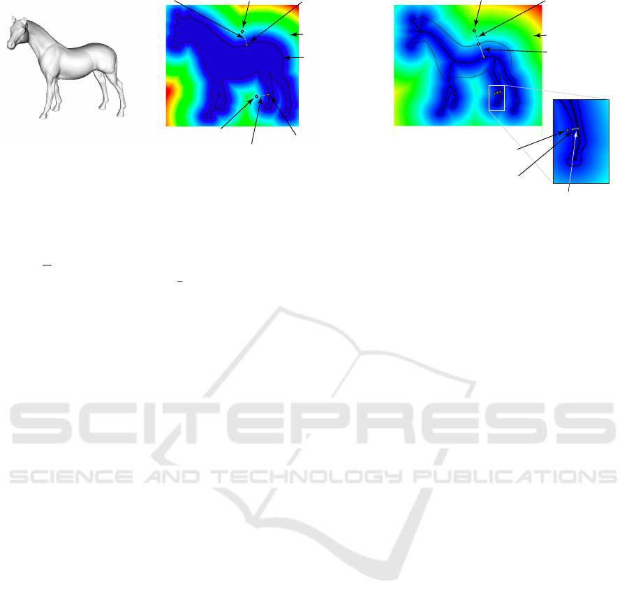
Selection Distance.

A third issue concerns the po-

sition of the point

that initiates the rotation: If one

clicks too far from the silhouette

Ω

, the rotation axis

may not match what one expects. To address this, we

forbid the rotation when the distance

from

Ω

exceeds a given upper limit

max

. That is, if the user

clicks too far from any silhouette in the viewport, the

rotation mechanism does not start. This signals to the

user that, to initiate the rotation, she needs to click

closer to a silhouette.

We compute

Ω

(p)

, where

Ω

is the view-

point area outside

Ω

, i.e., all viewport pixels where

Ω

near

equals the default Z buffer value (see Sec. 3.1A).

We studied two methods for estimating

max

(see

Fig. 5). First, we set

max

to a ﬁxed value, in practice

10% of the viewport size. Using a constant

max

however not optimal: We found that, when we want

to rotate around thick shape parts, such as the horse’s

rump in Fig. 5b, it is intuitive to select

even quite

far away from the silhouette. This is the situation of

point

in Fig. 5b. In contrast, when we want to

rotate around thin parts, such as the horse’s legs, it is

not intuitive to initiate the rotation by clicking too far

away from these parts. This is the situation of point

in Fig. 5b. Hence,

max

depends on the scale of the

shape part we want to rotate around; selecting large

parts can be done by clicking farther away from them

than selecting small parts.

We model this by setting

max

to the local shape

thickness (see Fig. 5c). We estimate this thickness

as follows: Given the clicked point

, we ﬁnd the

closest point to it on the silhouette boundary

∂ Ω

Interactive Axis-based 3D Rotation Speciﬁcation using Image Skeletons

173

sihouette

boundary ∂Ω

siho

boun

clicked point p

closest silhouette

point q

to p

distance to silhouette d

clicked point p

distance to silhouette d

closest silhouette

point q

to p

distance field DT

clicked point p

closest silhouette

point q

to p

distance field DT

shape thickness

at q

closest silhouette

point q

to p

clicked point p

shape thickness at q

Figure 5: Improvements of axis-based rotation method. (a) A view of the shape to be rotated. (b) Fixed maximum-distance

setting for two clicked points p

and p

. (c) Thickness-based maximum-distance setting for two clicked points p

and p

q = FT

Ω

(p)

. The shape thickness at location

is the

distance to the skeleton, i.e.,

Ω

(q)

. Here, the point

is the farthest clickable point around the location

to the silhouette that allows initiating a rotation around

the rump. If we click further from the silhouette than

the distance

max

from

, no rotation is done.

For the leg part, the farthest clickable point around

the location

has, however, to be much closer to

the silhouette (see Fig. 5c), since here the local shape

thickness, i.e., the distance

max

from

, is much

smaller.

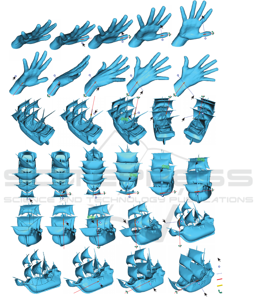
4 RESULTS

Figure 6 shows our 3D skeleton-based rotation applied

to two 3D mesh models. For extra insights, we rec-

ommend also watching the demonstration videos (The

Authors, 2019). First, we consider a 3D mesh model

of a human hand (100K faces), which is not water-

tight (open at wrist). We start from a poor viewpoint

from which we cannot easily examine the shape (a).

We click close to the thumb (b) and drag to rotate

around it (b-e), yielding a better viewpoint (e). Next,

we want to rotate around the shape to see the other

face, but keeping the shape roughly in place. Using

a trackball or world-coordinate axis rotation cannot

easily achieve this. We click on a point close to the

shape-part we want to keep ﬁxed during rotation (f),

near the the wrist, and start rotation. Images (g-j) show

the resulting rotation.

Figure 6(k-ad) show a more complex ship object

(380K polygons). This mesh contains multiple self-

intersecting and/or disconnected parts, some very thin

(sails, mast, ropes) (Kustra et al., 2014). Comput-

ing a 3D skeleton for this shape is extremely hard

or even impossible, as Eqn. 1 requires a watertight,

non-self-intersecting, connected shape boundary

∂ Ω

Our method does not suffer from this, since we com-

pute the skeleton of the 2D silhouette of the shape.

We start again from a poor viewing angle (k). Next,

we click close to the back mast to rotate around it,

showing the ship from various angles (l-o). Images

(p-u) show a different rotation, this time around an

axis found by clicking close to the front sail, which

allows us to see the ship from front. Note how the

2D skeleton has changed after this rotation – compare

images (p) with (v). This allows us to select a new

rotation axis by clicking on the main sail, to see the

ship’s stern from below (w-z). Finally, we click on the

ship’s rump (aa) to rotate the ship and make it verti-

cal (ab-ad). The entire process of three rotations took

around 20 seconds.

Figure 7 shows a different dataset type – a 3D

point cloud that models a collision simulation be-

tween the Milky Way and the nearby Andromeda

Galaxy (Dubinski, 2001; J. Dubinski et al., 2006). Its

160K points describe positions of the stars and dark

matter in the simulation. Image (a) uses volume ren-

dering to show the complex structure of the cloud,

for illustration purposes – we do not use this render-

ing in our method. Rather, we render the cloud in our

pipeline using 3D spherical splats (b). Image (c) shows

the cloud, rendered with half-transparent splats, so that

opacity reﬂects local point density. Since we render a

3D sphere around each point, this results in a front and

back buffer

Ω

near

and

Ω

f ar

, just as when rendering a

3D polygonal model. From these, we can compute

the 2D skeleton of the cloud’s silhouette, as shown in

the ﬁgure. Images (d-f) show a rotation around the

central tubular structure of the cloud, which reveals

that the could is relatively ﬂat when seen from the last

viewpoint (f). Image (g) shows the new 2D skeleton

corresponding to the viewpoint after this rotation. We

next click close to the upper high-density structure (f)

GRAPP 2020 - 15th International Conference on Computer Graphics Theory and Applications

174

(a) (b) (c) (d) (e)

(f) (g) (h) (i) (j)

click

drag

click

drag

(k) (l) (m) (n) (o)

click

drag

(p) (q) (r) (s) (t) (u)

click

drag

click

drag

click

drag

(v) (w) (x) (y) (z)

(aa) (ab) (ac) (ad)

Legend

pointer

clicked point p

pointer move d

rotation axis a

3D neighbors N

rotation direction

Figure 6: Examples of two rotations (a-e), (f-j) for the hand shape and four rotations (k-o), (p-u), (v-z), (aa-ad) for the ship.

and rotate around it. Images (h-j) reveal a spiral-like

structure present in the lower part of the cloud, which

was not visible earlier. To explore this structure bet-

ter, we next click on its local symmetry axis (l) and

rotate around it. Images (l-n) reveal now better this

structure. As for the earlier examples, executing these

three rotations took roughly 15 seconds. Scientists

involved with studied this dataset for roughly a decade

appreciated positively the ease of use of the skeleton-

based rotation as compared to standard trackball and

multi-touch gestures.

Interactive Axis-based 3D Rotation Speciﬁcation using Image Skeletons

175

(b) (c) (d) (e) (f)

click

drag

click

drag

click

drag

(g) (h) (i) (j)

(k) (l) (m) (n)

(a)

Figure 7: Exploration of astronomical point cloud dataset. (a) Volume-rendered overview (J. Dubinski et al., 2006). Rotations

around three 3D axes (b-f), (g-j), (k-n).

5 DISCUSSION

We next outline our method’s advantages and limita-

tions:

Ease of Use.

We can rotate around 3D axes locally

aligned with the scene’s features with a single click

and optionally pointer drag motion. This makes our

method usable to contexts where no second button,

modiﬁer keys, or multi-touch input is available. Find-

ing the axis works with even inexact click locations

as we use a set of closest 2D-skeleton points for that

(N(s

), Sec. 3).

Genericity.

We handle 3D meshes, polygon soups,

and point clouds; our only requirement is that these

generate fragments with a depth value. This contrasts

using 3D curve skeletons for interaction, which heav-

ily constrain the input scene quality, and cannot be

computed in real time, as already mentioned.

Novelty.

To our knowledge, this is the ﬁrst time

when 2D image-based skeletons have been used to

perform interactive manipulations of 3D shapes. Com-

pared to view-based reconstructions of 3D curve skele-

tons from their 2D silhouettes (Kustra et al., 2013),

our method requires a single viewpoint to compute an

approximate 3D curve skeleton.

Simplicity and Speed.

Our method consists of ba-

sic OpenGL 1.1 operations (primitive rendering and

Z-buffer reading) plus the 2D image-based skeletoniza-

tion method in (Ersoy et al., 2011). This skeletoniza-

tion method delivers us the skeleton

Ω

, its regulariza-

tion

Ω

, and the feature transform

Ω

. This method

is efﬁciently implemented in NVidia’s CUDA and C++,

so it handles scenes of hundreds of thousands of poly-

gons rendered onto

1000

pixel viewports in a few

milliseconds on a consumer-grade GPU, e.g. GTX

660. Its computational complexity is linear in the num-

ber of silhouette pixels, i.e.,

O(|Ω|)

. This is due to the

fact that the underlying distance transform used has

the same linear complexity. For details on this, we

refer to the original algorithm (Cao et al., 2010).

Implementing the two improvements presented in

Sec. 3 is also computationally efﬁcient: The skele-

ton’s distance transform

Ω

is already computed

during the rotation axis estimation (Sec. 3.1C). The

distance

Ω

and feature transforms

Ω

require one

extra skeletonization pass of the background image

Ω

. All in all, our interaction method delivers frame

rates over 100 frames-per-second on the aforemen-

GRAPP 2020 - 15th International Conference on Computer Graphics Theory and Applications

176

tioned consumer-grade GPU. For replication purposes,

the full code of the method is provided online (The

Authors, 2019).

Limitations.

Since 3D rotation axes are computed

from 2D silhouette skeletons, rotations are not, strictly

speaking, invertible: Rotating from a viewpoint

with an angle

around a 3D local axis

computed

from the silhouette

Ω

leads to a viewpoint

in which,

from the corresponding silhouette

Ω

, a different axis

6= a

can be computed. This is however a problem

only if the user releases the pointer (mouse) button

to end the rotation; if the button is not released, the

computation of a new axis

is not started, so mov-

ing the pointer can reverse the ﬁrst rotation. Another

limitation regards the measured effectiveness of our

rotation mechanism. While our tests show that one can

easily rotate a scene around its parts, it is still unclear

which speciﬁc tasks are best supported by this rotation,

and by how much so, as compared to other rotation

mechanisms such as trackball. We plan to measure

these aspects next by organizing several controlled

user experiments in which we select a speciﬁc task

to be completed with the aid of rotation and quanti-

tatively compare (evaluate) the effectiveness of our

rotation mechanism as compared to other established

mechanisms such as trackball.

6 CONCLUSION

We proposed a novel method for specifying interac-

tive rotations of 3D scenes around local axes using

image skeletons. We compute local 3D rotation axes

out of the 2D image silhouette of the rendered scene,

using heuristics that combine the silhouette’s image

skeleton and depth information from the rendering’s

Z buffer. Specifying such local rotation axes is simple

and intuitive, requiring a single click and drag ges-

ture, as the axes are automatically computed using

the closest scene fragments rendered from the current

viewpoint. Our method is simple to implement, us-

ing readily-available distance and feature transforms

provided by modern 2D skeletonization algorithms;

can handle 3D scene consisting of arbitrarily complex

polygon meshes (not necessarily watertight, connected,

and/or of good quality) but also 3D point clouds; can

be integrated in any 3D viewing system that allows ac-

cess to the rendered Z buffer; and works at interactive

frame-rates even for scenes of hundreds of thousands

of primitives. We demonstrate our method on sev-

eral polygonal and point-cloud 3D scenes of varying

complexity.

Several extension directions are possible as follows.

More cues can be used to infer more accurate 3D curve

skeletons from image data, such as shading and depth

gradients. Separately, we plan to execute a detailed

user study to measure the effectiveness and efﬁciency

of the proposed skeleton-based 3D rotation for speciﬁc

exploration tasks of spatial datasets such as 3D meshes,

point clouds, and volume-rendered data.

REFERENCES

Bade, R., Ritter, F., and Preim, B. (2005). Usability com-

parison of mouse-based interaction techniques for pre-

dictable 3D rotation. In Proc. Smart Graphics (SG),

pages 138–150.

Bian, S., Zheng, A., Chaudhry, E., You, L., and Zhang, J. J.

(2018). Automatic generation of dynamic skin defor-

mation for animated characters. Symmetry, 10(4):89.

Cao, T.-T., Tang, K., Mohamed, A., and Tan, T.-S. (2010).

Parallel banding algorithm to compute exact distance

transform with the GPU. In Proc. ACM SIGGRAPH

Symp. on Interactive 3D Graphics and Games, pages

83–90.

Chaouch, M. and Verroust-Blondet, A. (2009). Alignment

of 3D models. Graphical Models, 71(2):63–76.

Dubinski, J. (2001). When galaxies collide. Astronomy Now,

15(8):56–58.

Dufﬁn, K. L. and Barrett, W. A. (1994). Spiders: A

new user interface for rotation and visualization of

N-dimensional point sets. In Proc. IEEE Visualization,

pages 205–211.

Emory, M. and Iaccarino, G. (2014). Visualizing turbulence

anisotropy in the spatial domain with componental-

ity contours. Center for Turbulence Research Annual

Research Briefs, pages 123–138.

Ersoy, O., Hurter, C., Paulovich, F., Cantareiro, G., and

Telea, A. (2011). Skeleton-based edge bundling for

graph visualization. IEEE TVCG, 17(2):2364 – 2373.

Guo, J., Wang, Y., Du, P., and Yu, L. (2017). A novel multi-

touch approach for 3D object free manipulation. In

Proc. AniNex, pages 159–172. Springer.

Hesselink, W. H. and Roerdink, J. B. T. M. (2008). Eu-

clidean skeletons of digital image and volume data in

linear time by the integer medial axis transform. IEEE

TPAMI, 30(12):2204–2217.

J. Dubinski et al. (2006). GRAVITAS: Portraits of a universe

in motion. https://www.cita.utoronto.ca/

∼

dubinski/

galaxydynamics/gravitas.html.

Jackson, B., Lau, T. Y., Schroeder, D., Toussaint, K. C., and

Keefe, D. F. (2013). A lightweight tangible 3D inter-

face for interactive visualization of thin ﬁber structures.

IEEE TVCG, 19(12):2802–2809.

Kaye, D. and Ivrissimtzis, I. (2015). Mesh alignment using

grid based PCA. In Proc. CGTA), pages 174–181.

Kustra, J., Jalba, A., and Telea, A. (2013). Probabilistic

view-based curve skeleton computation on the GPU.

In Proc. VISAPP. SCITEPRESS.

Interactive Axis-based 3D Rotation Speciﬁcation using Image Skeletons

177

Kustra, J., Jalba, A., and Telea, A. (2014). Robust segmenta-

tion of multiple intersecting manifolds from unoriented

noisy point clouds. Comp Graph Forum, 33(4):73–87.

Reniers, D., van Wijk, J. J., and Telea, A. (2008). Computing

multiscale skeletons of genus 0 objects using a global

importance measure. IEEE TVCG, 14(2):355–368.

Rodrigues, R. S. V., Morgado, J. F. M., and Gomes, A.

J. P. (2018). Part-based mesh segmentation: A survey.

Comp Graph Forum, 37(6):235–274.

Rosenfeld, A. and Pfaltz, J. (1968). Distance functions in

digital pictures. Pattern Recognition, 1:33–61.

Siddiqi, K. and Pizer, S. (2008). Medial Representations:

Mathematics, Algorithms and Applications. Springer.

Sobiecki, A., Yasan, H., Jalba, A., and Telea, A. (2013).

Qualitative comparison of contraction-based curve

skeletonization methods. In Proc. ISMM. Springer.

Tagliasacchi, A., Delame, T., Spagnuolo, M., Amenta, N.,

and Telea, A. (2016). 3D skeletons: A state-of-the-art

report. Comp Graph Forum, 35(2):573–597.

Tangelder, J. W. H. and Veltkamp, R. C. (2008). A survey of

content based 3D shape retrieval methods. Multimedia

Tools and Applications, 39(441).

Telea, A. (2011). Feature preserving smoothing of shapes

using saliency skeletons. In Proc. VMLS, pages 136–

148. Springer.

Telea, A. and van Wijk, J. J. (2002). An augmented fast

marching method for computing skeletons and center-

lines. In Proc. VisSym, pages 251–259. Springer.

The Authors (2019). Source code and videos of interactive

skeleton-based axis rotation. http://www.staff.science.

uu.nl/

∼

telea001/Shapes/CUDASkelInteract.

Yu, L. and Isenberg, T. (2009). Exploring one- and two-

touch interaction for 3D scientiﬁc visualization spaces.

Posters of Interactive Tabletops and Surfaces.

Yu, L., Svetachov, P., Isenberg, P., Everts, M. H., and Isen-

berg, T. (2010). FI3D: Direct-touch interaction for the

exploration of 3D scientiﬁc visualization spaces. IEEE

TVCG, 16(6):1613–1622.

Zhao, Y. J., Shuralyov, D., and Stuerzlinger, W. (2011).

Comparison of multiple 3D rotation methods. In Proc.

IEEE VECIMS, pages 19–23.

GRAPP 2020 - 15th International Conference on Computer Graphics Theory and Applications

178