Deep-learning in Identification of Vocal Pathologies

Felipe L. Teixeira

and João P. Teixeira

1,2,*

Instituto Politécnico de Bragança (IPB), Bragança 5300, Portugal

Research Centre in Digitalization and Intelligent Robotics (CEDRI), Applied Management Research Unit (UNIAG),

Bragança 5300, Portugal

Keywords: Vocal Acoustic Analysis, Leave-one-out, Deep Neural Network, Architecture of Deep-NN, Dysphonia,

Vocal Fold Paralysis, Laryngitis Chronica.

Abstract: The work consists in a classification problem of four classes of vocal pathologies using one Deep Neural

Network. Three groups of features extracted from speech of subjects with Dysphonia, Vocal Fold Paralysis,

Laryngitis Chronica and controls were experimented. The best group of features are related with the source:

relative jitter, relative shimmer, and HNR. A Deep Neural Network architecture with two levels were

experimented. The first level consists in 7 estimators and second level a decision maker. In second level of

the Deep Neural Network an accuracy of 39,5% is reached for a diagnosis among the 4 classes under analysis.

1 INTRODUCTION

Voice is a sound resulting from a set of events in the

vocal apparatus and along the vocal tract, with a

certain force, sound, duration, speed and rhythm,

subconsciously regulated by the information sent

from the brain (Panek, Skalski, Gajda, &

Tadeusiewicz, 2015).

The vocal acoustic analysis allows quantifying

some characteristics of a sound signal. Using this

technique for the study of voice, it is possible, in a

non-invasive way, to determine and quantify the

vocal quality of the individual through the different

acoustic parameters that make up the signal

(Guimarães, 2004).

Only the self-parameters obtained with the vocal

acoustic analysis are not very conclusive, however, if

they are properly associated with an Artificial

Intelligence (IA) tool, the results are considerably

better (Guimarães, 2004; Matuck, 2005; Teixeira J. P.

et al, 2017)

The tools of IA are, therefore, an added value to

take into account, since analyzing a large number of

data, with several variables, it becomes difficult for

the human being. After performing the training of an

IA system, it is expected that the system be able to

generalize. This means, for a new situation, never

seen before, the system should be able to make a

decision based on similar parameters seen before

(Teixeira F., et al, 2018; Guedes et al, 2019).

A Deep Learning technic is based on the so-called

artificial neural network. However, they have a

greater number of hidden layers in their architecture,

which helps in the processing of information and it

can still have different activation functions in each

hidden layer. The purpose of additional hidden layers

is to have some more objective but non-final ‘image’

of the output.

In this work it was intended to do the same study

that Teixeira F. et al (2018) did, however, instead of

Support Vector Machine, a Deep Learning approach

is used.

The main objective of this work is to distinguish

between pathological and healthy subjects and to

distinguish the different pathologies under study.

In this work, three groups of subjects were used.

Subjects with Dysphonia, Vocal Fold Paralysis and

subjects with the Laryngitis Chronica

 pathology.

These diseases are the ones that most often cause

disturbances in the human voice (University, 2018),

being sometimes undetectable to the human ear.

Dysphonia is a disorder of the voice, often caused

by abnormalities that affect the vibration of the vocal

chords. This affects the ability to speak easily and

clearly. Dysphonia is characterized by the symptoms

of hoarseness, weak voice, changes in voice tone and

it may arise suddenly or gradually (Teixeira J. P. &

Fernandes P. O., 2015).

Laryngitis Chronica consists of an inflammation

that can result from inhalation of irritants or by the

intensive use of voice. Symptoms include gradual

288

Teixeira, F. and Teixeira, J.

Deep-learning in Identiﬁcation of Vocal Pathologies.

DOI: 10.5220/0009148802880295

In Proceedings of the 13th International Joint Conference on Biomedical Engineering Systems and Technologies (BIOSTEC 2020) - Volume 4: BIOSIGNALS, pages 288-295

ISBN: 978-989-758-398-8; ISSN: 2184-4305

loss of voice, hoarseness, and sore throat (Huche, F.,

& Allali, A., 2005; Kumar et al., 2010).

Paralysis of the Vocal Folds is the total

interruption of the nervous impulse. Being this total,

it happens in the two Vocal Folds, or being partial,

occurs only in one of the Folds. This situation can

occur at any age and the problems associated with this

condition correspond to voice change, respiratory

problems and swallowing problems.

For the analysis, the following parameters are

used: relative jitter, relative shimmer, Harmonic to

Noise Ratio (HNR), Noise to Harmonic Ratio (NHR),

Autocorrelation and Mel Frequency Cepstral

Coefficients (MFCC). These parameters were

extracted from sustained vowels /a/, /i/ and /u/ in high,

low and normal tones. The MFCC’s were also

extracted from continuous speech.

Next section describes the used methodologies. In

this section, the parameters are presented, the

materials used are identified and the methodology,

based on deep neural network, is also presented. The

section 3 presents the results and discussion. Finally,

the last section summarizes the work developed and

the conclusions.

2 MATERIAL AND

METHODOLOGY

The parameters used in this work combine source

parameters that are related with vocal folds and

therefore with low frequency components (jitter,

shimmer, HNR and Autocorrelation), with

parameters related with vocal folds and vocal tract,

spreading a large bandwidth of frequencies (MFCCs).

The first set of parameters were extracted from a

sustained speech of vowel. The MFCCs were

extracted both from the same vowels but also from

continuous speech.

The parameter used were just retrieved from the

cured database (Fernandes, J. et al, 2019) with the

parameters extracted from the Saarbrucken Voice

Database (SVD) as detailed below. This cured

database contains only the subjects diagnosed with

just one pathology/condition, been rejected all

subjects with more than one pathology/condition.

The speech samples were classified into 4 classes

(3 pathologies/conditions and control) using one

Deep Artificial Neural Network with architecture

projected for this specific purpose.

2.1 Parameters

For this work, it was necessary to extract a set of

parameters from acoustic speech files to build the

cured database of speech parameters (Fernandes, J. et

al, 2019). These parameters are relative jitter, relative

shimmer, HNR, NHR, Autocorrelation and 13

MFCC’s.

The jitter analysis for a speech signal is the mean

absolute difference between consecutive periods,

divided by the mean period and expressed as a

percentage (Eq. 1).



1

∑

|













|



∑









100,

(1)

where T

is the length of the glottal period i, and N

the number of glottal periods.

The relative shimmer is defined as the mean

absolute difference between magnitudes of

consecutive periods, divided by the mean amplitude,

expressed as a percentage (Eq. 2).



1

∑















|



∑









100,

(2)

where A

is the magnitude of the glottal period i,

and N the number of glottal periods.

The HNR is a parameter in which the relationship

between harmonic and noise components provides an

indication of overall periodicity of the speech signal

by quantifying the relationship between the periodic

component (harmonic part) and aperiodic (noise)

component. The overall HNR value of a signal varies

because different vocal tract configurations imply

different amplitudes for harmonics. HNR can be

given by Eq. 3.

10





1

,

(3)

where H is the normalized energy of the harmonic

components and 1-H is the remaining energy of signal

considered the non-periodic components (noise).

In the autocorrelation function, the similarity of

periods along the signal is evaluated. The greater the

similarities, the greater the autocorrelation value

(Guedes et al, 2019).

According to (Fernandes J. et al, 2018),

mathematically the autocorrelation can be determined

in 3 steps.

In the first step (equation 4), having a signal x(t)

uses a segment of the same signal of duration T,

centered on tméd. From the selected part, the average

Deep-learning in Identiﬁcation of Vocal Pathologies

289

of μx is subtracted and the result is multiplied by a

window function w(t) to obtain a signal window:









é









(4)

The window function w(t) is symmetrical around t

and 0 everywhere outside the time interval [0, T].

(Boersma, 1993) mentions that the window must be a

sine or Hanning window, given by equation 5.

=12−12 2

(5)

Then the normalized autocorrelation ra(



) of the

selected signal part is calculated (equation 6). This is

a symmetrical function of delay τ:

ra





ra



τ

















τ

























(6)

Finally, it is necessary to calculate the normalized

autocorrelation rw(τ) of the window function used.

Using the Hanning window, autocorrelation is

obtained through equation 7.

rw





1







cos

2τ







2



2



(7)

To estimate the autocorrelation rx(τ) of the

original signal segment, the autocorrelation ra(τ) of

the signal window is divided by the autocorrelation

rw(τ) of the window used (Eq.8).

rx























,

(8)

where ra(t) is the normalized autocorrelation of

the signal and rw(t) is the normalized autocorrelation

of a window used.

Therefore, the autocorrelation function of a

sustained speech signal displays the local maxima for

multiples of τ, so it is only necessary to identify the

first local maxima, which will correspond to the

harmonic part.

The NHR parameter quantifies the relationship

between the aperiodic component (noise) and the

periodic component (harmonic part). Although it is

the inverse of HNR, it is not measured in the

logarithmic domain, so the values are not the inverse

(Fernandes, J. et al, 2018). The NHR parameter can

be given by equation 9.















1

1

(9)

The MFCC’s parameters are based in the

spectrogram of the signal. The extract process can be

divided in 7 steps (Lindasalwa Muda, 2010).

The first step (Pre-Emphasis) is to emphasize the

higher frequencies by increasing the signal energy at

these same frequencies. The calculation for Pre-

Emphasis is given by equation 10 where x[n] is the

speech signal.

















 0,95



1



(10)

The second step (Framing) consists of dividing the

signal into small frames, where it is advised that each

frame should be between 20 and 40 milliseconds. The

third step (window) is to multiply a window function

by each frame of the signal.

In the fourth step, it is necessary to convert the N

samples of each frame from the time domain to the

frequency domain, using the discrete Fourier

transform (Lindasalwa Muda, 2010).

Equation 11 is used for its calculation, where X(k)

are the spectral coefficients, x(n) the signal frame. It

should be noted that the values of n and k must be

greater than or equal, to zero and less than or equal,

to N-1.

























,





(11)

The fifth step serves to make the transformation to

the Mel scale.

To make this transformation, equation 12 is used.

In this process, triangular filters are applied to the

spectrum to make the conversion.









2595∗







700

1,

(12)

In the sixth stage comes the discrete cosine

transform, which consists in transforming the Mel

spectrum into the time domain. This transformation

can be referred to as Mel Frequency Cepstrum

Coefficient, where the lowest order coefficients

represent the vocal tract shape and the higher order

coefficients represent the waveform periodicity

(Lindasalwa Muda, 2010; Tiwari, V., 2010).

Finally, in the last step the signal energy of a signal

is calculated for a segment at time t1 to time t2 using

equation 13.

y=

[]

(13)

In this work 13 MFCC were used, and the first

coefficient is the energy of the signal.

BIOSIGNALS 2020 - 13th International Conference on Bio-inspired Systems and Signal Processing

290

2.2 Materials

In this work, we used the German Saarbrucken Voice

Database (SVD) (Barry, W.J., Pützer, n.a.) to extract

the parameters associated with the various subjects

used for the study. In this database is possible to find

more than 2000 subjects. For each subject it is

available a recording for 3 sustained vowels (/a/, /i/,

/u/) in three different tones. There is also the German

phrase: ”Guten Morgen, wie geth es Ihnen?” (Good

morning, how are you?). The sampling frequency of

voice signals is 50 kHz. The file size is between 1 and

3 seconds with a resolution of 16 bits.

Subjects with Dysphonia, Laryngitis Chronica and

Vocal Fold Paralysis were used because they are the

pathologies with higher number of subjects. Subjects

with more than one pathology/condition were

rejected.

The parameters were extracted for 473 subjects,

according to the groups shown in table 1.

In the work of (Teixeira J. P. et al., 2018) it was

proved that there is no difference between the male

and female gender for the parameters relative jitter,

relative and absolute shimmer, HNR, NHR and

autocorrelation for control subjects and Laryngitis

Chronica subjects. Therefore, there was no separation

made by gender.

The subjects available in SVD limited the size and

mean age of each pathological group.

Table 1: Dataset ages by each pathologic group and control

group.

Groups

Sample

size

Average

age

Standard

deviation

of ages

Control 194 38,1 14,4

Dysphonia 69 47,4 16,4

Laryngitis

Chronica

41 49,7 13,5

Vocal Fold

Paralysis

169 57,8 13,8

Total 473

For every subject the parameters were extracted

from sustained vowels, and the MFCC’s parameters

were also extracted from the continuous speech

sentence. Three groups of parameters were organized.

The first group contains only parameters related with

the source. This group I, actually was structured into

group I(a) and I(b).

Group I(a) contains the parameters Jitter, Shimmer

and HNR for the 9 vowels by subject, in a total of 27

features.

The group I(b) contains the parameters Jitter,

Shimmer, HNR, NHR and Autocorrelation for the 9

vowels by subject, in a total of 45 features.

The group II contains the 13 MFCC’s extracted

from the 9 sustained vowels, in a total of 117 features

by subject.

The group III contains 13 MFCC’s extracted from

50 overlapped segments of the continuous speech, in

a total of 650 features by subject.

The jitter and shimmer parameters were extracted

using the algorithm developed by Teixeira and

Gonçalves (2016). The HNR, NHR, Autocorrelation

and MFCC’s parameters were extracted with the

work developed by Fernandes J. et al (2019).

2.3 Deep Learning Architecture

The basic structure of the developed architecture is to

have two levels. The first level consists in a set of

multi-layer-perceptron neural networks (NN). Each

one will give a guess if the sample corresponds to the

class 1, class 2 or none (3 output classes). The 4

classes (3 pathologies and control) were combined

into 6 NN. One additional NN were considered to

classify between control/pathologic, only with binary

classification. Therefore, the first level consists into 7

NN, presented in Table 2. The organizations of NN

with 3 classes were used to allow the use of the all

dataset to trains each NN.

The second level consists in a NN with 7 nodes in

the input, hidden layers, and one output. The input

receives the output of the 7 NN of first level. The

output is the classification of one of the 4 classes.

Figure 1 presents a representation of the Deep NN

developed.

It is expected that each NN of first level be

specialized in the classification between two

pathologies. The second level would receive the

guess of this 7 specialized NN and take a final

decision.

Table 2: Neural Networks for first level of Deep Learning.

N N 1 Healthy / Pathological

N N 2 Healthy / Dysphonia / Other

N N 3 Healthy / Laryngitis / Other

N N 4 Healthy / Paralysis / Other

N N 5 Dysphonia / Paralysis / Other

N N 6 Dysphonia / Laryngitis / Other

N N 7 Laryngitis / Paralysis / Other

Deep-learning in Identiﬁcation of Vocal Pathologies

291

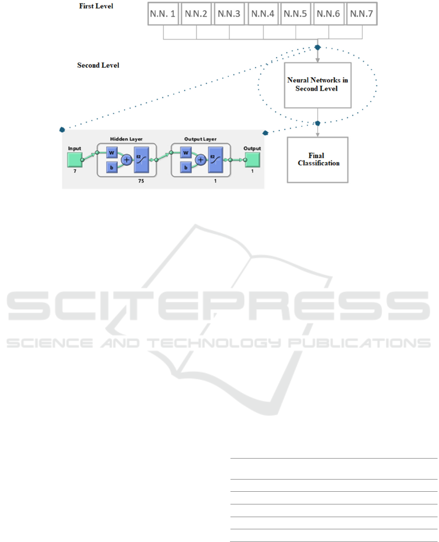
Figure 1: Deep Learning architecture.

For each parameters group, different NN

Architectures were experimented.

The best architecture for the second level was

achieved experimentally. It has 7 nodes in input layer

(outputs of first level), 75 nodes in hidden layer and

the training function is Levenberg-Marquardt

(Marquardt, D., 1963).

The second level of Deep- Learning is responsible

for classify the pathology of each subject. It is

possibel classify between four classes, three

pathological and one healthy.

The number of hiddden layer were also

experimented. One architecture with 2 hidden layer,

where the second layer had 4 nodes has expected to

achieve better acuracy, suposing that each of this 4

nodes will classify one of the 4 classes. But the

experimental result did’t show what was expected.

3 RESULTS AND DISCUSSION

The “leave-one-out” method has implemented to train

the Deep-NN. This method consists of testing all

subjects, performing as many training sessions as

subjects exist in the sample size. In N session of

training, N-1 subjects were used to train and the

remaining used to test. At the end, the all subjects

were tested and never were used in the train process.

This methodology is a time consuming process but

allows using larger number of subject to train and to

test.

The result presented was measured for the subject

in the test.

3.1 First Level

Table 3 show the results for the NN of the first level

to classify between control/pathologic, using the tree

groups of parameters. Acc is the Accuracy, Pre is the

Precision, Sen corresponding to Sensibility, Spe is the

Specificity and F1 corresponding to F1-Score. It can

be seen that the higher accuracy is 72.7% using the

parameters of group I(a).

Table 4 shows the results obtained in one of the

remaining 6 NN of first level as example

(Healthy/Paralysis/Others). The result for the

remaining 5 NN has similar numbers. The measures

are presented grouping the 3 output classe into groups

of two classes to allow the determination of the all

measures presented.

It can be seen that parameters of group I(a) achive

again, generally, higher accuracy.

Table 3: Measured values to classify healthy / pathological

subjects.

Group of

Parameters

I(a) I(b) II III

Acc (%)

72.7 72.3 67.2 71

Pre (%)

69.6 68 53 57.2

Sen (%)

65.9 65.7 61.7 67.3

Spe (%)

78 77.2 70.3 73

67.7 66.8 57 61.8

BIOSIGNALS 2020 - 13th International Conference on Bio-inspired Systems and Signal Processing

292

Table 4: Obtained values for classification between Healthy/Paralysis/Others with the different parameter groups.

Healthy / Paralysis / Others

Parameters Group I (a) Group I (b) Group II Group III

Healthy / Others

Accuracy (%) 61,3 58,2 54,6 59

Precision (%) 41,2 32,5 36 46,9

Sensibility (%) 74,8 80,8 62,5 65,5

Specificity (%) 55,6 51,7 51,2 55

F1 53,2 46,3 45,8 54,7

Paralysis / Others

Accuracy (%) 63,7 60,8 59,2 60,5

Precision (%) 60,1 71,1 67,4 63,1

Sensibility (%) 45 37,9 35,5 38,5

Specificity (%) 81,2 84,2 82,8 80

F1 54,5 49,4 46,5 47,8

Others / (Healthy +

Paralysis)

Accuracy (%) 49 43,6 45,3 49,8

Precision (%) 60,9 69,1 63,6 55,5

Sensibility (%) 26,2 24,9 25,7 26,4

Specificity (%) 78,4 78,9 76,5 76,1

F1 36,6 36,6 36,7 35,8

3.2 Complete Deep-NN

As mentioned previously, “Leave-one-Out” method

has used, therefore, each subject was classify by eight

neural networks (seven in first level and one in second

leve), this process was repeat 473 times (number of

subjects).

Table 5 presents the accuracy of the complete

Deep-NN using three alternatives for the number of

nodes in the hidden layer of the second level. It also

presents the time consuming to train and test the all

dataset using the “Leave-one-out” method. This

values was obtained with processor Intel ®

i5-

3337u CPU@ 1.80GHz.

Table 5: Accuracy obtained and time consuming for the

Deep-NN.

Nodes in

hidden layer

Accuracy (%) Time (minutes)

50 30.4 141.1

75 39.5 168.5

80 36.4 116.4

Table 5 shows the best accuracy to classify

between the 4 classes is 39,5% using 75 nodes in the

hidden layer.

Table 6 presents the confusion matriz for the best

classification situation. The column of ‘Target’

corresponding the real situation of the subject, in

‘Classification’ line is mentioned the Deep-NN

classification. The diagonal line has the number of

subjects correctly classified. Where H is the Healthy

subjects, D the Dysphonia, L the Laryngitis and P

corresponds to Paralysis.

The confusion matriz shows that there is no

problem with unbalance of the dataset.

Table 6: Confusion matrix.

Classification

H D L P

Target

H 98 62 27 7

D 20 21 13 15

L 9 13 8 11

P 24 38 47 60

Deep-learning in Identiﬁcation of Vocal Pathologies

293

3.3 Discussion

Although several methodologies was tried, this article

only contain the best results achieved.

The results shown that the neural network is a

promising tool for voice pathology classification. In

the work presented in (Teixeira F,, Fernandes J.,

Guedes V., Junior A., & Teixeira J. P., 2018) the

Support Vector Machines (SVM’s) was used to

classify between control/pathologic with the same

dataset with best results about 70% accuracy.

Comparing with present results of the first level NN

an accuracy of about 73% was achieved,

demonstrating the improvements introduced using

ANN.

Guedes et al, 2019 developed a system to classify

between the same 4 classes but using parameters from

continuous speech and using transfer-learning

technics to do the classification. Very similar results

was achieved, with F1-score of 40% for classify

between four categories.

No separation by gender was used because for

Laryngitis Chronica it was reported in (Teixeira J. P.

et al., 2018) no gender difference for the relative

jitter, relative and absolute shimmer, HNR, NHR and

Autocorrelation. Anyhow, other conditions like

Dysphonia and Vocal Fold Paralysis was used, and

maybe some gender difference can exist for these

subjects. Therefore, it is recommended to experiment

a gender separation in future work.

4 CONCLUSIONS

This article describes the experience of using neural

networks for diagnosis between healthy subjects and

subjects with one of the three pathologies under study

(Laryngitis Chronica, Dysphonia or Vocal Fold

Paralysis). The parameters used in this analysis were

extracted from sustained vowels or from a sentence.

A Deep NN was developed in two levels to

classify between 4 classes.

The best results in the first level between

control/pathologic subjects were an accuracy of 73%.

The best results between the 4 classes in the

second level was an accuracy of about 40%.

The best results, in some cases, were not obtained

with the same parameters group, however generally

de parameters of group I(a) demonstrate the best

results in higher number of cases. Therefore, for the

uniformity reasons it was considered that group I(a)

is the best group of parameters experimented. These

parameters are relative jitter, relative shimmer and

HNR.

As a final conclusion, the accuracy of about 40%

to make the identification between healthy subjects

and 3 pathologies still below the requirements to

became a real application. These results demand more

research on this type of classification, experimenting

different models of classification, different type of

features, more subjects and maybe gender separation.

ACKNOWLEDGEMENTS

This work has been supported by FCT – Fundação

para a Ciência e Tecnologia within the Project Scope:

UIDB/5757/2020.

REFERENCES

Barry, W.J., Pützer, M. Saarbrücken Voice Database,

Institute of Phonetics, Univ. of Saarland, http://www.

stimmdatenbank.coli.unisaarland.de/

Boersma, P., 1993. “Accurate short-term analysis of the

fundamental frequency and the harmonic-to-noise ratio

of a sample sound,” IFA Proceeding, vol. 17, pp. 97-

110.

Fernandes

J., Silva, L., Teixeira, F., Guedes

V., Santos, J.

& Teixeira, J. P., 2019. Parameters for Vocal Acoustic

Analysis - Cured Database. In Procedia Computer

Science – Elsevier.

Fernandes, J., Teixeira, F., Guedes, V. Junior, A. &

Teixeira, J. P. , 2018. “Harmonic to Noise Ratio

Measurement - Selection of Window and Length”,

Procedia Computer Science - Elsevier. Volume 138,

Pages 280-285.

Guedes, V.; Teixeira, F.; Oliveira, A.; Fernandes, J.; Silva,

L.; Junior, A. & Teixeira, J. P., 2019. Transfer Learning

with AudioSet to Voice Pathologies Identification in

Continuous Speech. Procedia Computer Science –

Elsevier.

Guimarães, I. (2004). Os Problemas de Voz nos

Professores: Prevalência, Causas, Efeitos e Formas de

Prevenção. 22.

Huche, F., & Allali, A. (2005). A Voz - Patologia vocal de

origem orgânica. (5th ed., Vol. 3; A. Editora, Ed.).

Kumar, V., Abbas, A. K., Fausto, N., & Aster, J. C. (2010).

Robbins and Cotran Patologia – bases patológicas das

doenças. (8 ed). Rio de Janeiro: Brasil: Elsevier Editora

Ltda.

Lindasalwa Muda, M. B., 2010. Voice Recognition

Algorithms using Mel Frequency Cepstral Coefficient

(MFCC) and Dynamic Time Warping (DTW)

Techniques. J. O. COMPUTING, Ed.

Marquardt, D. (1963). An Algorithm for Least-Squares

Estimation of Nonlinear Parameters. SIAM Journal on

Applied Mathematics, 11(2), 431-441.

BIOSIGNALS 2020 - 13th International Conference on Bio-inspired Systems and Signal Processing

294

Matuck, G. R. (2005). Processamento de Sinais De Voz

Padrões Comportamentais por Redes Neurais

Artificiais. São José dos Campos.

Panek, D., Skalski, A., Gajda, J., & Tadeusiewicz, R.

(2015). Acoustic Analysis Assement in Speech

Pathology Detection. Int. J. Appl. Math. Comput. Sci.

Teixeira, F., Fernandes, J., Guedes, V. Junior, A. &

Teixeira, J. P., 2018. Classification of

Control/Pathologic Subjects with Support Vector

Machines. Procedia Computer Science - Elsevier.

Volume 138, Pages 272-279.

Teixeira, J. P. & Fernandes, P. O., 2015. “Acoustic

Analysis of Vocal Dysphonia”. Procedia Computer

Science - Elsevier 64, 466 – 473.

Teixeira, J. P., Fernandes, J., Teixeira, F., Fernandes, P.,

2018. Acoustic Analysis of Chronic Laryngitis -

Statistical Analysis of Sustained Speech Parameters. In

Proceedings of the 11th International Joint Conference

on Biomedical Engineering Systems and Technologies,

pp 168-175.

Teixeira, J. P., Fernandes, P. O. & Alves, N. , 2017. “Vocal

Acoustic Analysis – Classification of Dysphonic

Voices with Artificial Neural Networks”, Procedia

Computer Science - Elsevier 121, 19–26.

Teixeira, J. P., Gonçalves, A., 2016. Algorithm for jitter and

shimmer measurement in pathologic voices. Procedia

Computer Science - Elsevier 100, pages 271 – 279.

Tiwari, V., 2010. MFCC and its applications in speaker

recognition. International Journal on Emerging

Technologies 1(1): 19-22(2010) ISSN: 0975-8364e t

University, H., 2018. Vocal fold Disorders. Harvard M.

School, Editor.

Deep-learning in Identiﬁcation of Vocal Pathologies

295