Self-organized Cognitive Algebraic Neural Network

Prabir Sen

Statgraf Research, Canada

Keywords: Artificial Intelligence, Cognitive Computation, Deep Neural Network, Decision Science, Network Science.

Abstract: This paper refers to author’s patented invention that introduces a more efficient statistical (machine)

learning method. Inspired by neuroscience, the paper combines the synaptic networks and graphs of quantum

network to constitute interactions as information flow. Hitherto, several machine learning algorithms had

some influence in business decision-making under uncertainty, however the dynamic cognitive states and

differences thereof, at different timepoints, play an important role in transactional businesses to derive choice

and choice-sets for decision-making at societal scale. In addition, deep neural functions that reflect the

direction of information flow, the cliques and cavities, necessitate a new computational framework and deeper

learning method. This paper introduces a proactive-retroactive learning technique - a quantified measurement

of a multi-layered-multi-dimensional architecture based on a Self-Organized Cognitive Algebraic Neural

Network (SCANN) integrated with Voronoi geometry – to deduce the optimal (cognitive) state, action,

response and reward (pay-off) in more realistic imperfect and incomplete information conditions. This

quantified measurement of SCANN produced an efficient and optimal learning results for individuals’

transactional activities and for nearest-neighbor, as a group, for which the individual is a member. This paper

also discusses and characterizes SCANN for those who handle decisions under conditions of uncertainty,

juxtaposed between human and machine intelligence.

1 INTRODUCTION

Human decision making routinely involves choice

among temporally extended courses of action,

response and reward, as pay-off, over a broad range

of time scales depending on cognitive state. Consider

a traveler deciding to undertake a journey to a distant

city for work. To decide – go-no-go – the end-benefits

in terms of reward, as pay-off, of the trip must be

weighed against the cost. Having decided to go,

choices must be made at each fragmented “smaller”

decision e.g., whether the work is worth paying or

not, whether to fly or to drive, whether arrange a local

accommodation or stay with friends or relatives. With

the brute force of computational processes and the

better understanding of human intelligence – how

individuals go about solving their problem – some of

the existing learning technologies may train machines

for the outcome. Here one would like to make a

distinction between precision engineering and

intelligence. One of the fundamental principles in

precision engineering is that of determinism where

systemic behavior is fully predictable, even to an

https://orcid.org/0000-0001-6436-5998

individual’s, or atomic-scale, activities. To do the job

efficiently and correctly, one needs models and

algorithms, where the basic idea is that machine

follows a set of rules, cause and effect relationships,

that are within human ability to understand and

control and that there is nothing random or

probabilistic about their behavior. Further, the

causalities are not esoteric and uncontrollable, but can

be explained in terms of familiar and precise

engineering principles. Intelligence, on the other

hand, as opposed to fact, is stochastic in nature. It

finds optimal solutions, derives reasons, infers

actions, recognizes patterns, comprehends ideas,

solves problems and uses language to communicate,

from (im)perfect and (in)complete information

conditions.

However, some learning methods, where the

result is the final reward or pay-off, are awfully hard

to untangle the future information to foresee the

sequence of actions that will benefit the user at some

point in future. Some of these infrequent and delayed

rewards or learnings limit decisions making process

(Edward, Isbell, Takanishi, 2016). For some

836

Sen, P.

Self-organized Cognitive Algebraic Neural Network.

DOI: 10.5220/0009141408360845

In Proceedings of the 12th International Conference on Agents and Artiﬁcial Intelligence (ICAART 2020) - Volume 2, pages 836-845

ISBN: 978-989-758-395-7; ISSN: 2184-433X

combinatorial problems, where all rules and

information are known to all parties, one may set up

intermediate positions for them to achieve the optimal

results where, as in real-life conditions, such learning

success depends on how well one would fragment a

“major” decision or an objective into a series of

multiple “smaller” decisions – the decision journey –

and actions to measure their progress accurately.

Unlike many statistical (machine) learning

techniques, this approach has yielded both

unreliability in the training process, and a general lack

of understanding as to how the learning model

converge, and if so, to what (Barnett 2018).

2 PROACTIVE-RETROACTIVE

Most humans or species do not learn by rote or by

reinforcing the subject into the memory. In fact, the

growth and maturation of a child’s brain is an

intricate process taking decades, in which the brain

grows and adapts to the surrounding world (Aamodt,

and Wang, 2008). The same research has shown that

the developing brain has been shaped by thousands of

generations of evolution to become the most

sophisticated information-processing machine on

earth. And, even more amazingly, it builds itself. The

way the information is processed can be termed as

dynamic proactive-retroactive learning wherein a

human (or a system) proactively learn, either through

instructions or through observations, and then waits

for some kind of confirmation – either from nearest-

neighbor or trusted source – which retroactively

reinforce or modify in accordance with the subject

matter. For example, when a child learns “A for

Apple, B for Boy and C for Cat” from a book, he or

she registers only an image of an apple, a boy or a cat.

These images are retained in memory until, some

point in future, when he or she physically observes

the contextual appearance – new information that

connects the dots – of an apple, or a boy or a cat, and

confirmed by a trusted source, often parents, with the

text – the name – associated with those physical

images. Even most adult brains follow the same

principle when they observe something new. At the

time of observation, they retain this new information

in their memory as postulations – “may be this is a

peach” (language text) or “may be the boy is playful”

(causal reasoning) or “may be this is Mr. Smith”

(personality), until their postulations are confirmed

by a trusted source, often in the nearest-neighbor.

These observations and confirmations happen in two

different time-points. And, sometimes the observed

postulations are radically altered with the

confirmation of new information – “oh no, this is an

apricot, not peach” (language text) or “no, the boy is

sarcastic, not playful” (causal reasoning) or “ah, this

is Mr. David, not Mr. Smith” (personality) – at the

time of confirmation. In this learning process, the

former is proactive learning whereas, the latter –

retroactive learning – changes the original

postulations or replaces the deep-seated beliefs

through new information connections, often either

guided by experience or information from the

nearest-neighbor or both (Sen, 2017).

So, what happens to state of the information

between proactive and retroactive – two different

time points – in the learning cycle? The neuroscience

research has shown that in early childhood, and again

in the teens and subsequently at various stages of

learning, brains go through bursts of refinement,

forming and then optimizing the connections in the

brain. Connections determine what the subject or

object is, what does it do, and how does it do. Early

childhood provides an incredible window of

opportunity with neural connections forming and

being refined at such an incredible rate, there isn’t a

certain time when babies are learning – they are

always learning. Every moment, each experience

translates into physical trace, a part of the brain’s

growing network (Bachleda and Thompson, 2018),

One of the most powerful set of findings concerned

with the learning process involves the brain’s

remarkable properties of “plasticity” – to adapt, to

grow in relation to experienced needs and practice,

and to prune itself when parts become unnecessary –

which continues throughout the lifespan, including

far further into old age than had previously been

imagined (Skoe and Kraus (2012). The demands

made on the human learning are key to the plasticity

– the more one learns, the more one can learn – and,

therefore required to be included in this architecture

of artificial neural network for machine learning.

3 NEURAL NETWORK WITH

VORONOI REGION

An effective method for designing neural network

that derives the stages in-between proactive and

retroactive learning in two different time points is to

classify patterns in the multi-dimensional feature

space. This deep learning architecture introduces a

multi-dimensional feature space where the

information waits in certain workspace – the Voronoi

region – within the neural network based on distance

to points in a specific subset of the plane. The

Self-organized Cognitive Algebraic Neural Network

837

Voronoi diagram is derived over points in feature

space which represents teachers’ input in order to

realize the desired classification. However, to reduce

the size of the neural network and make the learning

efficient, clustering procedure that enables the

subject to manage a number of teachers in a lump is

implemented (Kenji, Masakazu and Shigeru, 1999).

Our approaches, however, only utilize point-wise

cell-membership – as new information – by means of

nearest-neighbor queries and do not utilize further

geometric information about Voronoi cells since the

computation of Voronoi diagrams is prohibitively

expensive in high dimensions. Therefore, a Monte-

Carlo-Markov-Chain integration-based approach

(Polianskii and Pokorny, 2019) that computes a

weighted integral over the boundaries of Voronoi

cells, thus incorporates additional information – as

retroactive confirmation – about the Voronoi cell

structure is established. This dynamic proactive-

retroactive learning method predicts and prescribes

an action in “expected” response to an activity of

human (or interchangeably a machine), depending on

individual’s state, for one or more end-rewards, or

pay-offs at a given point in time.

Since most information related to immediate

relevance including dynamic active cognitive state

and/or active experiences, hence individuals apply a

certain set of rules that are associated with either

sequential monadic (e.g., individual’s state from a to

𝑎́ as self-improvement) or paired-comparison (e.g.,

individual’s state x compared with another

individual’s state y) with nearest neighbor or a group

where individual is a member. This, in imperfect or

asymmetric and incomplete information conditions,

creates “hidden” multi-layered combinations on

multi-dimensions – functional, non-functional, non-

discriminating and discriminating – features to

predict and determine the cognitive state (or “state”).

The group, where individual is a member, may also

apply a certain set of collective “hidden” information

associated with either linear-non-linear (e.g., a race-

car driver uses wind direction data while cornering at

speeds more than 200 mph without informing the

opponent) or paired comparison (e.g. race car the

team analyzes data of other racers’ degradation rates

on the tires and of the health of various mechanical

components, and recording the drivers’ steering,

braking and throttle inputs). In imperfect and

incomplete information conditions, this generates

aggregated “hidden” multi-layered combinations on

multi-dimensions features to predict and determine a

collective state. For example, a trading system

analyzes data to predict if the state of any trading

stock and its change with new features, conditions

and functions – the underlying latent variables –

affect the price, as an outcome, in the marketplace.

The hypotheses here are that the dynamic

proactive-retroactive learning method would derive

to be a better prediction on the individual’s current

action for future reward, as final pay-off, over a

broad range of time and information scales, including

(im)perfect and (in)complete information conditions.

For example, if the trading system predicts that the

state of the product (or service) and its change with

the underlying latent variables affect price in the

marketplace, then the expected response of the buyer

may also likely to change (either to buy immediately

or defer for the future price), thus may create a

different reward or pay-off outcome (revenue or

saving for the trader).

4 TRAINING DATA

A self-organized learning method, in accordance with

the dynamic proactive-retroactive learning method is

executed to segment a graph network data based on

bounded diffusion of collective individual

information interactions. The nearest-neighbor or

group data is determined from grouping of individual

transactional data for a group where individual is a

member. After a certain upper-bound number of

groups, the system applies a diffusion-limited

aggregation (“DLA”) – a formation process whereby

individuals in a group, as particles, and their signals

– defined as change or the first derivative in an

individual’s data – of a subject matter undergo a

stochastic process for clustering together to different

aggregates (“clusters”) of such individuals. These

signals and their changes – defined as the second

derivative in an individual’s data – are used for

predicting the group’s current state, as described

above, and applied sheafing method, (or group

theory) for “grouping” mechanism (Tennison, 2011)

– depending on the geometry of the growth, for

example, whether it be from a single point radially

outward or from a plane or line – of clusters where

the individual is a member, to determine the state.

The self-organized learning method presents

individual’s data, for example, as stimulus, at some

time t=0 and then presenting a response data at a

variable time post stimulus on the group. The

bounded diffusion in DLA, for example, may have

one additional parameter, the position of the decision

bound, say A. If at time t of the state data of the

individual (or subject matter e.g., search for an item)

is x, the distribution of the state at a future time may

be s > t, hence the term “forward” diffusion. The

ICAART 2020 - 12th International Conference on Agents and Artiﬁcial Intelligence

838

backward diffusion, on the other hand, may be useful

when the individual at a future time s has a particular

behavior due to past decision, the distribution at time

is t < s. This may impose a terminal condition, which

is integrated backward in time, from s to t (hence the

term “backward” is associated with this). Let g(x) be

a bounded smooth (twice continuously differentiable

having compact support) function, and let:

𝑢

(

𝑡,𝑥

)

=𝐸

,

(𝑔𝑋

(

𝑇

)

≡𝐸(𝑔𝑋

(

𝑇

)

|𝑋

(

𝑇

)

=𝑥

(1)

with the “terminal” condition u(T, x) = g(x). In

addition, if X(t) has a density p(t, x), then for a

probability density function μ(·), the probability

densities satisfy the:

𝜕

𝜕𝑡

𝑝

(

𝑡,𝑥

)

=(𝐴

∗

𝑝)(𝑡,𝑥)

(2)

where A* is the adjoint operator of A, defined as:

𝐴

∗

𝑣

(

𝑡,𝑦

)

=−

𝜕

𝜕𝑦

𝑏

(

𝑦

)

𝑣

(

𝑡,𝑦

)



𝜕



𝜕𝑦



(𝜎



(

𝑦

)

𝑣(𝑡,𝑦)

(3)

This behavior may be described as fractal growth,

as frequently observed in plants like ferns. The

clusters may include formulating a group associated

with the group’s current activity as well as the

nearest-neighbor for the individual where individual

is a member.

These state data of individual are used to predict

the group’s current action where the individual is a

member, to determine the choice clusters of likely

action. The action data are further used to predict the

group’s expected response to formulate choice

clusters of likely response. And, finally, these

response data are used to predict the group’s reward

or pay-offs to derive choice clusters of the reward or

pay-off in their decision journey.

5 COGNITIVE ALGEBRAIC

NEURAL NETWORK

A multi-layered multi-dimensional Self-Organized

Cognitive Algebraic Neural Network (“SCANN”)

learning method is formulated, in accordance with

the dynamic proactive-retroactive learning method

and self-organized learning method. This is required

to arrange information and determine undefined rules

based on a cognitive structure for the individual (or

the subject matter). This may include choices and

maximum likelihood estimation of each choice for

the activity of the individual. A set of data in activity,

for example, is determined for each individual (n) and

more individuals are added to the activity content that

form choices and different choice sets. The features

(or attributes) of these choices and choice-sets may or

may not be causal factors that influence a choice. A

choice set attribute may comprise one or more

attributes, for example, of the item such as

combination of sensory attributes, (taste, looks, etc.),

rational (price, ingredients, etc.) and emotional (feel

good, lifestyle, etc.). In the formation of a group with

different clusters, based on activity and/or factors

thereof, each choice set becomes a function of

activity and interactions within a group, where the

individual is a member. One or more common

contact individual and/or individual’s activity content

between individuals may exist in a group. Further,

this indicates a “hub” contact with “cross” features

and attributes for individual and/or individual’s

activity content between individuals in a group, thus

forms a graph structure of the network.

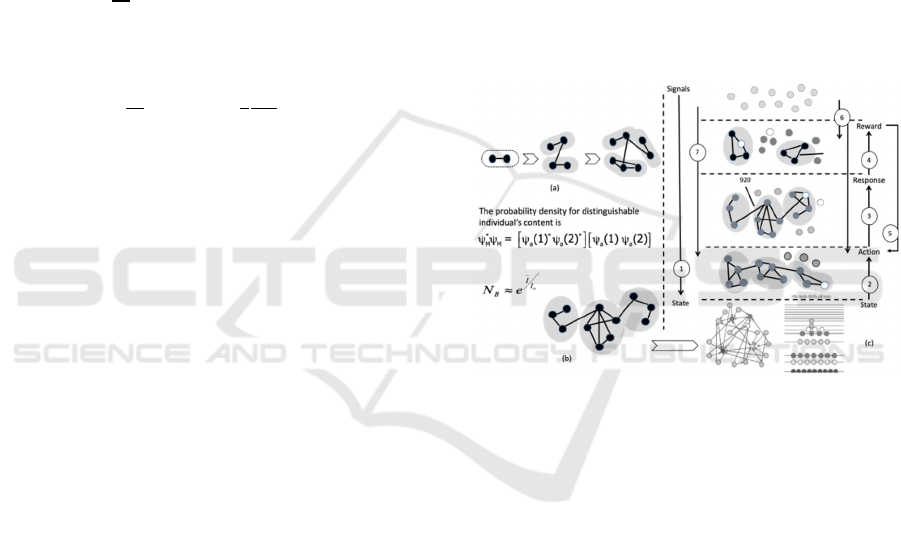
Figure 1: Multi-Layered Multi-dimensional Self-Organized

Cognitive Algebraic Neural Network (SCANN).

The graph structure of the SCANN is a pair (N,

g), where g is a network on the set of nodes N. A

relationship between two nodes i and j, represented

by 𝑖𝑗 ∈ 𝑔, is referred to as a link or edge. Thus, g

will sometimes be an 𝑛 × 𝑛 adjacency matrix, with

entry 𝑔



denoting whether i is linked to j and may

also include the intensity of that relationship. The

neighbors of a node i in a network (N, g) are denoted

by N

(g). The degree of a node i in a network (N, g)

is the number of neighbors that i has in the network,

so that 𝑑



(g) =

𝑁



(g)

. Many naturally occurring

multi-layered multi-dimensional networks (Erdös,

and Renyi, 1960), as represented in this Fig 1,

explicitly incorporate multiple channels of

connectivity and constitute the natural environment

to describe systems interconnected through different

categories of connections: each activity content

module (signals, states, actions, responses and

rewards) may be represented by a layer and the same

Self-organized Cognitive Algebraic Neural Network

839

node or entity may have different kinds of

interactions (set of nearest-neighbors in each layer).

The latent feature structure, as depicted in Fig. 1

above, is abstracted from variables to render

microstate probabilities of each (dis)satisfied

individual’s choice-set attributes and latent causal

variables, accessible by mere combinatorial,

(im)perfect and (in)complete information conditions

much in the same way as graph probabilities, become

accessible in random graph. At an atomic level, for

each individual, the structure finds the optimal

choice-set of latent variables that has causal effect on

the expected outcome or reward or pay-off (Sen,

2015). The interaction variables that are available for

individuals to exercise preference, or any variable

involving an interaction of the individual for a good

or service. The coefficients are predetermined and

represented a diminishing level of satisfaction, for

example, over time. In addition, the latent learning

represents that, in cognitive decision, despite their

non-equilibrium and irreversible nature, the evolving

network is mapped into an equilibrium Bose-Einstein

(“BE”) condensation nodes corresponding to energy

levels, and links representing the individual’s activity

contents, as particles (Bianconi and Barabási, 2001).

The existence of a state transition, phase to a BE

condensate, the outcome distribution g

(

)

= C ∈



where 𝜃 is a free parameter and the energies were

chosen from ϵ ∈ (0, 𝜖



) with normalization

C= 𝜃+ 1/(𝜖





). For this class of distributions, the

cognitive state for a Bose condensation is determined

as:

𝜃+1

(𝛽𝜖



)



𝑑𝑥

𝑥



𝑒



−1









()

(4)

The active strand of the study in this direction is

to study individualized ensembles with fixed degree

sequences, or degree distributions following, for

instance, a power-law. This is the probability that a

randomly chosen node in the network has exactly 𝑙

links, is proportional to 𝑙



for some y .

The choices for individuals (or interchangeably

machines) in N have action spaces A

. Let A =

𝐴



,…𝐴



at every stage in their decision journey. In

this, the action spaces are finite sets or subsets of a

Hilbert space. Generally, decision making is not

necessarily associated with a choice of just one action

among several simple given options, but it involved

a choice between several complex options for

actions. The elementary prospect (e

) is the

conjunction of the chosen modes, one for each action

from the intended action. To each elementary

prospect e

, there corresponds the basic state

𝑒



⟩

which is a complex function 𝐴



→ 𝐶, and its

Hermitian conjugate

⟨

𝑒



. The structure of a basic

state is

⟨

𝑒

𝑛

=⨂

𝑖=1

𝑁

𝐴

𝑖𝑣

𝑖

(5)

The cognitive or mind space is the closed linear

envelope

𝑀≡span

{

𝑒



⟩

}

𝑁

⨂

𝑖=1

𝑀



(6)

To each prospect πj, there corresponds a state

𝜋



 ∈ 𝑀 that is a member of the mind space.

𝜋



=

∑

𝑎



𝑒



⟩

. This applies a quantum decision

theory as an intrinsically probabilistic procedure. The

first step consists in evaluating, consciously and/or

subconsciously, the probabilities of choosing

different prospects from the point of view of their

usefulness and/or appeal to the choosing agent. If the

mapping from a state parameter w to the conditional

probability density p(y|x, w) is one-to-one, then the

model is identifiable, i.e. if the product in service is

in its lowest state then the likelihood of that product

to fail is significantly high. Otherwise, it is non-

identifiable. In other words, this model is identifiable

if and only if its parameter is uniquely determined

from its state and/or cognitive behavior.

However, in non-identifiable cases, as depicted in

Fig. 1, actions are more dynamic and remain in active

workspace of the individual as they “wait” – the

Voronoi region – for more signals in transactional

data to make the connection for action (best matching

nearest-neighborhood action cells). For these non-

identifiable cases of actions, a new set of information

is required, as new cell, ∁ , and a local counter

variable 𝜏

∁

that constrains the number of input

signals for which the action has best-matching unit

(Fukushima, 2013). Further, introduction of a new

signal data, as a new cell, ∁, with a local counter

variable 𝜏

∁

and since the cells are slightly moving

around, more recent signals may be weighted

stronger than previous ones. An adaptation step, for

example, may be formulated as: a) choose an input

signal data according to the probability distribution

𝑃(𝜉), b) locate the best matching unit 𝑐=∅



(

𝜉

)

; c)

increase matching for 𝑐 and its direct topological

neighbors ∆𝑤



=𝜀



(𝜉− 𝑤



) ; d) Increment the

signal counter of 𝑐, as new signal data gets added,

either via another activity, e.g., a call from a friend,

or an ‘autonomous’ message: “how about going out

for lunch” : ∆𝜏



=1; e) decrease all signal counters

by a fraction 𝛼 : ∆𝜏

∁

=−𝛼𝜏

∁

(not shown in the

diagram) which is uniquely determines the change in

action due to new signal data that influenced its state

),2( ∝∈

ICAART 2020 - 12th International Conference on Agents and Artiﬁcial Intelligence

840

and/or cognitive behavior. The relative signal

frequency of a cell ∁ is: ℎ



=𝜏



∑

𝜏

∈

. A high

value of ℎ



, therefore, indicates a good position to

insert a new latent variable, as cell, because the new

latent variable, cell, is likely to reduce this high value

of action to a certain degree. The insertion of new

cells leads to a new Voronoi region, F, in the input

space. At the same time, the Voronoi regions of the

topological neighbors of ∁ are diminished. This

change is reflected by an according redistribution of

the counter variables 𝜏

∁

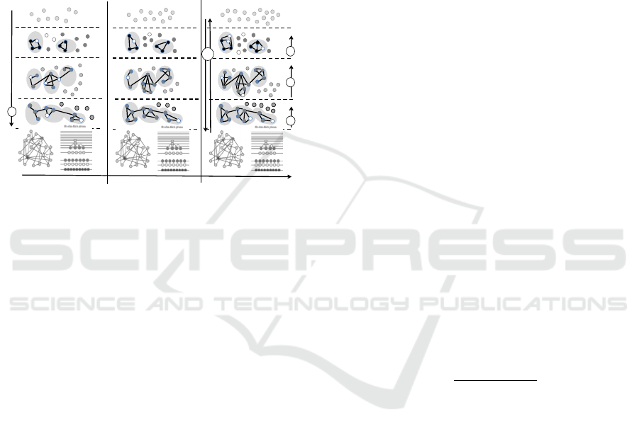
Figure 2: Self-Organized Cognitive Algebraic Neural

Network (SCANN) With Voronoi Region.

There are also many conditions where the

individual and/or individuals in a group choose

actions without fully knowing with whom they will

interact and what would be their response. Instead of

a fixed network, individuals are now unsure about the

network that will be in place in the future, but have

some idea of the number of interactions that they will

have. To fix ideas, the individual and/or a group

where individual is a member and their action data

may choose to find expected response that is only

useful in interactions with other individuals who has

the same product as well, but without being sure of

with whom one will interact in the future. In

particular, the set of individuals N is fixed, but the

network (N; g) is unknown when individuals choose

their actions. An individual i knows his or her own

degree d

, when choosing an action, but does not yet

know the realized network. Individuals choose

actions in {0,1}, individual i has a cost of choosing

action

, denoted c

. Individual i’s payoff from action

when i has d

neighbors and expects them each

independently to choose 1 with a probability x is:

𝑣

(

𝑑



,𝑥

)

−𝑐



and so action

is an expected response

for individual i if and only if 𝑐



≤ 𝑣(𝑑



,𝑥). The

payoff to the individual from taking action

compared

to action

depends on the number of neighbors who

choose action

, so that

𝑠𝑖𝑔𝑛



𝑢



1,𝑎





(

)

−𝑢



0,𝑎





(

)





𝑠𝑖𝑔𝑛

∑

𝑎

∈



(

)

−

∑

1−𝑎

∈



(

)

 (7)

If more than one half of i's neighbors choose

action

, for example, then it is best for individual i to

choose 1, and if fewer than one half of i’s neighbors

choose action

then it is best for individual i to choose

action

. There may be multiple equilibria in this

situation. In non-identifiable cases of expected

response may be dynamic and/or in active workspace,

as the expected response data of the individual

“wait” for more signal data or action data to make

connection for expected response or lack of

confidence (best matching neighborhood action cells)

on the existing signal data. The prospect probability

may be defined as: 𝑝𝜋



,𝜏=Τ𝑟







(

𝜏

)

𝑃



(𝜋



The interaction of the decision maker with the group

may ensure that the individual keeps distinct identity

and personality while, at the same time, possibly

changing state of mind. In other words, the

surrounding group does influence the individual’s

state, but does so in a way that does not suppress the

person making own decisions. This corresponds to

the behavior of a subsystem that is part of a larger

system that changes the subsystem properties, while

the subsystem is not destroyed and retains its typical

features.

Introduction of a new signal data, as in Fig 2, or

action data as a “new” cell, ∁, with a local counter

variable 𝜏

∁

and since the cells are slightly moving

around, more recent signals may be weighted

stronger than previous ones. Here, the changes of the

signal and action counters as redistribution of the

counter variables may be seen as ascribing to the new

cell. This new cell is connected to the existing

expected response cells in such a way that may again

a structure consisting only of k-dimensional

simplices:

∆𝜏

∁

𝐹

∁



−𝐹

∁





𝐹

∁





(8)

A new Voronoi region exists now. As much input

signals and/or actions as it would have received if it

had existed since the beginning of the process. In the

same way the reduction of the counter variables of its

neighbors may be motivated by making more

information available to all. In such network

interactions the possible outcomes of the D and C to

two basis vectors

𝐷

⟩

and

𝐶

⟩

in the space of a two-

state condition, e.g., either coffee (A) or juice (B), the

state of the situation may be described by a vector in

the product space which could be spanned by the

basis

𝐶𝐶

⟩

𝐶𝐷

⟩

𝐷𝐶

⟩

and

𝐷𝐷

⟩

, where the first and

second entries refer to A’s and B’s states,

respectively. This may denote the responses initial

state by

𝜓



⟩

= 𝐽



𝐶𝐶

⟩

, where 𝐽



is a unitary operator

which may be known to both individuals. For fair

response, 𝐽



must be symmetric with respect to the

Reward

Response

Action

State

Time Horizon

State

Signals

Self-organized Cognitive Algebraic Neural Network

841

interchange of the two individuals. The strategies are

executed on the distributed pair of state situations in

the state

𝜓



⟩

. Strategic moves of two individuals,

for example, A and B are associated with unitary

operators 𝑈





and 𝑈





, respectively, which are chosen

from a strategic space S. The independence of the

individuals dictates that 𝑈





and 𝑈





operate

exclusively on the states in A’s and B’s possession,

respectively. The strategic space S may therefore be

identified with some subset of the group of unitary 2

x 2 matrices. Having executed their moves, which

leaves the situation in a state 𝑈





⨂𝑈





𝐽



𝐶𝐶

⟩

, A and

B forward their states for the final measurement

which determines their payoff. The only strategic

notion of a payoff may be the expected payoff. A’s

expected payoff may be given by



=𝑟𝑃



+𝑝𝑃



+𝑡𝑃



+𝑠𝑃



(9)

where 𝑃



=

⟨

𝜎𝜎′𝜓



 is the joint probability

that the channels 𝜎 and 𝜎′. A’s expected payoff $

not only depends on her choice of strategy 𝑈





, but

also on B’s choice 𝑈





Individual i’s reward or payoff function may be

denoted u

: 𝐴× 𝐺(𝑁) → ℝ. A given individual's

payoff depends on the group where the individual is

a member or other individuals' actions, but only on

those to whom the individual is (directly) linked in

the network. In fact, without loss of generality the

network may be taken to indicate the payoff

interactions in the group. More formally, individual’s

payoff may depend on a

and {𝑎



}

∈

(g)

so that for

any i, a

, and g: 𝑢



(𝑎





,g) = 𝑢



(𝑎



,á



,g) whenever



= á



for all 𝑗 𝜖 𝑁



(g). Unless otherwise indicated

the equilibrium, may be a pure strategy Nash

equilibrium: a profile of actions a ∈ 𝐴 = 𝐴



…𝐴



, such that 𝑢



(𝑎





,g) ≥ 𝑢



(𝑎



́ ,a



,g) for all

𝑎́



∈𝐴



. In the case with large fluctuations in input of

expected response with large-scale networks,

however, the weights increase without limits due to

the diffusion effect if weight constraints are absent.

Nevertheless, the choice probability of a network

with diverging weights asymptotically approaches

matching behavior. A weight-normalization

constraint may be imposed for the diffusion effect to

become more evident than in cases without

normalization.

However, in non-identifiable cases of reward

may be in dynamic and/or active workspace, as the

reward data of the individual “waits” for more signal

data or action data or expected response data to make

connection for reward or lack of confidence (best

matching neighborhood action cells) on the existing

signal data.

Introduction of a new signal data, or action data

or expected response data as a new cell, ∁, with a

local counter variable 𝜏

∁

and since the cells are

slightly moving around, more recent signals may be

weighted stronger than previous ones. Here the main

characteristic of the model could be that several

adaptation steps may sometimes be followed by a

single insertion. One may note the following

feedback relation between the two types of action: a)

every adaptation step may increase the signal, action

and response counters of the best-matching unit and

thereby increases the chance that another cell will be

inserted near this cell; b) insertion near a cell ∁

decreases both the size of its Voronoi field 𝐹

∁

and the

value of the signal or action or expected response

counter. The reduction of the Voronoi field makes it

less probable that ∁ will be best-matching unit for

future input signals.

Networks are then analyzed in terms of groups of

nodes that are all-to-all connected, termed as cliques.

The number of neurons in a clique determines its size,

or more formally, its dimension. In directed graphs it

is natural to consider directed cliques, which are

cliques containing a single source neuron and a single

sink neuron and reflecting a specific motif of

connectivity (Song, Sjöström, Reigl, Nelson and

Chklovskii, 2005), wherein the flow of information

through a group of neurons has an unambiguous

direction. The manner in which directed cliques bind

together can be represented geometrically. When

directed cliques bind appropriately by sharing

neurons, and without forming a larger clique due to

missing connections, they form, termed as, cavities

(“gaps,” “voids” or “unknowns”) in this geometric

representation, with high-dimensional cavities

forming when high-dimensional (large) cliques bind

together. Directed cliques describe the flow of

information in the network at the local level, while

cavities provide a global measure of information flow

in the whole network. Using these naturally arising

structures, we established a direct relationship

between the structural graph and the emergent flow

of information in response to stimuli, as captured

through time series of functional graphs (Reimann,

Nolte, Scolamiero, Turner, Perin, Chindemi, Dlotko,

Levi, Hess and Markram, 2017).

These structural graphs are analyzed at different

timepoints. As time progresses, for example, the

parameters in rules associated with active experience

or historical or neither may change and/or eliminated,

and thereby change prediction and prescription that

determine the action data for the action indicator. As

time progresses, at each step of determining the state

data, the action data, the expected response data, and

ICAART 2020 - 12th International Conference on Agents and Artiﬁcial Intelligence

842

the reward data also change optimal controls for the

individual and groups. The Voronoi region 𝐹

∁

, for

example, by an n-dimensional hypercube with a side

length equal to the mean length 𝑙

∁

of the edges

emanating from ∁ with 𝑙

∁

computed by

𝑙

∁

𝑐𝑎𝑟𝑑 (𝑁

∁

)





‖

𝑤

∁

−𝑤



‖

∈

∁

(10)

From the above, it is evident that it would be very

helpful to know the true dimensionality of the data,

meaning the smallest dimensionality t, such, that a t-

dimensional sub-manifold of V may be found

containing all (or most) input data. Then t-

dimensional hyper-cubes may be used to estimate the

size of the Voronoi regions. However, to figure out

the value of t, especially because the mentioned sub-

manifold may not have to be linear but could be

randomly twisted. Therefore, even analyses of the

signal, state, expected response and reward data may

not, in general, reveal their true dimensionality and

remain “unaided”, but gives only (or at least) an

upper bound. However, the method of training for

machine to learn and, therefore, gives some general

rules for choosing such an estimate that do work well

for all activities that may be encountered

subsequently.

Moreover, as time progresses, the learning

system may accelerate or decelerate the speed of

information flow between signal and state and action,

and expected response and reward. This may support

the two structural update operations: a) insertion of a

cell, as a neuron; b) deletion of a cell, as a neuron.

These operations may be performed such that the

resulting structure consists exclusively of multi-

dimensional structure ℋ . Although such a data

structure may already be sufficient in this example, a

considerable search effort may be needed to make

consistent update operations. The removal of a cell

may also require other neurons and connections are

removed to make the structure consistent again.

Simple heuristics as, for example, to remove a node

remove all neighboring connections and the node

itself may not work properly. For this purpose, a

tracking mechanism of all the ℋ may be introduced

in the current network. Technically, a new data type

simplex may be created, an instance of which

contains the set of all nodes belonging to a certain ℋ.

Furthermore, with every node associated to the set of

those ℋ the node may be part of. The two update

operations can now be formulated as: a) a new node

r may be inserted by splitting an existing edge qf. The

node r may be connected with q, f, and with all

common neighbors of q and f. Each ℋ containing

both q and f (in other words, the edge being split) may

be replaced by two ℋ each containing the same set

of nodes as ℋ except that q respectively f may be

replaced by the new node r. Finally, the original edge

qf may be removed. The new ℋ may be inserted in

the sets associated with their participating nodes. b)

to delete a node, it may be necessary and sufficient to

delete all ℋ the node may be part of. This may be

done by removing the ℋ from the sets associated

with their nodes. The same may be done with nodes

having no more edges. This strategy may lead to

structures with every edge belonging to at least one

ℋ and every node to at least one edge. Therefore, the

resulting k-dimensional structures may be consistent,

that is, contain only k-dimensional ℋ.

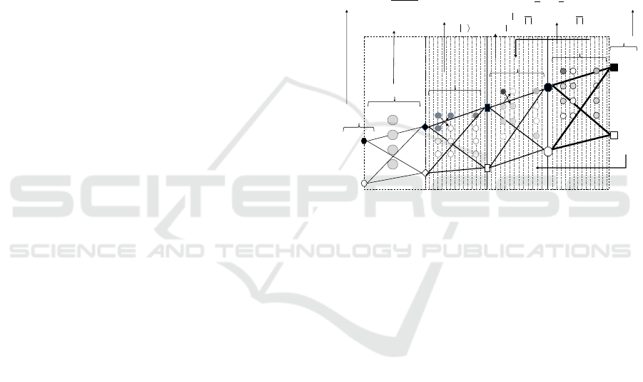
Figure 3: Optimal Learning of SCANN With Voronoi

Regions Derive Choice-sets.

Fig. 3 above illustrates an optimization method of

multiple-layered multi-dimensional with dynamic

expansion and contraction of SCANN structure – the

plasticity – where the individual activity content, as

structured in the learning system, are optimized with

dynamic programming method to minimize statistical

errors. A relational clique is constructed of a

clique over all activities at various locations on a

trajectory, which has an activity of one or more

individuals. Each clique C is associated with a

potential function 𝜙



(

𝑣



)

that maps a tuple (values

of decisions or aggregations). These evolutionary

structures may establish a relationship between the

structural graph and the emergent flow of information

in response to activity content, as captured over time

of functional graphs. The activity content and

likelihood of (K-1) dimensional simplex 𝑆



in the

network structure may find multi-nomial distribution,

which could be denoted as Mult(𝑝



,… 𝑝



; 𝑛), in a

discrete distribution over K dimensional non-

negative integer vectors 𝐱∈ℤ





where

∑

𝑥







= 𝑛.

Here, 𝒑 = (𝑝



;…;𝑝



) in an element of 𝑆



and 𝑛 >

1. Together they may provide a) activity-content, b)

probability mass function as expressed,

…

Signal (k)

Signals Group (K)

Signals in activity (ξ

)

Individual (i)

…

Individuals Group (l)

Actions in activity ( )

Hidden factors(g

)

Response in activity(sr)

…

Individuals in

activity (I

)

…

u= 1…A

Reward in activity(u

)

…

State in activity (s

)

…

Latent features (a

)

State (Z)

Action (A)

…

Latent attributes (w

)

Response (B)

State in Group (Z’)

Action in Group (A’)

Response in Group (B’)

Reward (U)

Reward in

Group (U’)

Group in

activity (I’

)

f (x

,..., x

; p

,..., p

, n) =

Γ(n+1)

Γ(x

+1)

i=1

∏

i=1

∏

(t) = c

k=0

−1



(t) + d

j, k

k=0

−1



j= j

∞



j, k

(t)



 =

∈

(

∈

)



−

∈

(

∈

)

(

⊗

)

JCC

(

)



(

)

−



(

)

(

)

a,i

(t +Δt) = 1−

Δt













a,i

(t) +

a, j

(t)



j≠i















cc ∈

Self-organized Cognitive Algebraic Neural Network

843

𝑓

(

𝑥



,…,𝑥



; 𝑝



,…𝑝



,𝑛

)

Γ(𝑛 +1)

∏

Γ(𝑥



+1)





𝑝











(11)

to optimize activity content for the individual with

minimized errors. For example, the buyer’s system in

a buyer-seller-trader network optimizes the product

information workspace that may wait for additional

information to formalize specific rules, say “predict”,

and minimize errors.

Any new or update on activity content may

initiate signals in activity, which may form the

maximum likelihood estimate (“MLE”) of the signal

and noise (e.g. data not immediate relevance) for

imperfect or incomplete information condition

parameters may train machine to learn as a signal, as

well as the MLE of the noise parameters may be

trained to be learned as noise. The ratio of these two

quantities may be taken and compared with upper and

lower thresholds until a decision may be made, based

on two properties desirable in a continuous sequential

detection which may have no analogue in fixed-

sample detection, or even in sequential detection, and

optimized content as in

𝜉

(

𝑡

)

=𝑐





,



∅





,

(

𝑡

)











+𝑑

,











𝜓

,

(𝑡)







(12)

First, the likelihood ratio could be a continuous

function of the length of the observation interval for

fixed parameter estimates; second, the MLEs could

also be continuous functions of the observation

interval.

Each individual signal data, as quantum

candidate, are aggregated into groups as a function of

one or more of attributes and features including time,

location, transition and constraints. The grouping

included an aggregation of each individual’s

decisions into groups, based on sheafing methods

used earlier for the aggregation into groups for

systematically tracking each individual’s signal data,

with various attributes and features, attached to open

sets of a topological space. We fix a set Λ of values

for a latent variable. A latent-variable model ℎ over

Λ assigns, for each 𝜆∈Λ and ∁ ∈ ℳ, a distribution

ℎ

∁



∈ 𝒟

ℛ

ℰ(∁). It also assigns a distribution ℎ



∈

𝒟

ℛ

(Λ) on the latent variables. This may obtain the

map ℰ

(

𝑋

)

⟶∏

∁∈ℳ

𝒫(ℰ

(

∁

)

) . We may use the

isomorphism

𝒫(𝑋





)≅

𝒫

(𝑋





)

(13)

which may take the limit of the cohomology

groups of the neural network system as

𝐻



(

{

𝑈



→𝑈

}

,𝐹

)

= ker (Hom

⨁



𝑍





,𝐹⇉

Hom



⨁

,

𝑍



,

,𝐹



= HomZ

{



}

,𝐹 (14)

The groups determined by grouping methods use

prediction activities and optimization of content

operation for the groups. Based on the predictions for

the group, an optimal set of choices may be

determined for the group. For example, in the trading

system of buyer-seller-trader network optimizes the

product information workspace for the aggregated

group to “forecast” price of nearest-neighbor, predict

maximum likelihood of forecasted price of the

nearest-neighbor and minimize errors to formalize

specific rules and optimal policies for various

features and attributes that drive forecast.

This abstraction of dynamic and active

workspace, as layer, created for each optimized

signal data including “wait” data and “new cell”

data, as explained above, parallel connections

between any cliques and cavities as described above,

as sigma cell in the layer (l) and the output of any

data, as neuron, in the layer (l

-1

) may be generated.

The number of these parallel connections is equal to

the number of activation functions in the layer (l).

Therefore, in the layer (l) an activation function along

with all sigma cells or equivalently the sigma blocks

are considered as a single multi-dimensional data or

neuron, as shown by dashed line in Fig. 3.

6 CONCLUSIONS

Multi-layered and multi-dimensional SCANN

networks explicitly incorporate multiple channels of

connectivity and constitute the natural environment to

describe decision-making system interconnected

through different categories of connections: each

channel (relationship, activity, category) is

represented by a layer and the same node or entity

may have different kinds of interactions (different set

of neighbors in each layer).

In addition, when SCANN is used, a smaller error

rate of about 0.32% can be acquired with a much

smaller number of reference vectors, if the SCANN is

combined with tune-up Voronoi region (Vr). The

computational cost of this method is smaller not only

for deep learning but also for the pattern recognition

due to smaller number of reference vectors.

The future research will study the interaction

structures of economic or knowledge networks

accounts for cognitive intelligence, if any, that require

SCANN methods. The study will emphasize the

properties of perfect and complete information; the

ICAART 2020 - 12th International Conference on Agents and Artiﬁcial Intelligence

844

interaction of potential use of SCANN; and the

exponentiality of the deeper neural network.

REFERENCES

Edwards, Ashley; Isbell, Charles; Takanishi, Atsuo (2016):

Perceptual Reward Functions; Frontiers and Challenges

Workshop, IJCAI 2016.

Barnett, Samuel A (2018): Convergence Problems with

Generative Adversarial Networks; A dissertation

presented for CCD Dissertations on a Mathematical

Topic, Mathematical Institute, University of Oxford

2018.

Aamodt, Sandra and Wang, Sam (2008): Welcome to Your

Brain: Why You Lose Your Car Keys But Never Forget

How to Drive and Other Puzzles of Everyday Life; New

York, USA.2008.

Sen, Prabir (2017): Data Analysis and Rendering, Patent

Application No. 15/789,216 Publication No. US-2019-

0122140-A1.

Bachleda, Amelia R. and Thompson, Ross A. (2018): How

Babies Think; Zero to Three, January 2018.

Skoe, Erika and Kraus, Nina (2012): A Little Goes a Long

Way: How the Adult Brain Is Shaped by Musical

Training in Childhood; The Journal of Neuroscience,

August 22; 32(34):11507–11510.

Kenji Amaya, Masakazu Endo, Shigeru Aoki (1999):

Construction of Neural Network using Cluster Analysis

and Voronoi Diagram; Transactions of the Japan

Society of Mechanical Engineers Series C, 1999;

Volume 65 , Issue 638.

Polianskii, Vladislav and Pokorny, Florian T. (2019):

Voronoi Boundary Classification: A High-Dimensional

Geometric Approach via Weighted Monte Carlo

Integration; Proceedings of the 36th International

Conference on Machine Learning, Long Beach,

California, PMLR 97, 2019.

Tennison, B.R (2011): Sheaf Theory; Cambridge

University Press 1975.

Erdo¨s, P. & Renyi, A (1960). On the evolution of random

graphs. Publ. Math. Inst. Hung. Acad. Sci. 5.

Sen, Prabir (2015): Location-based Cognitive and

Predictive Communication System; US Patent

9,026,139.

Bianconi, G., and Barabási, A.L., (2001): Bose-Einstein

Condensation in Complex Networks; Phys. Rev. Lett.

86, 5632 – Published 11 June 2001.

Fukushima, K (2013): Artificial Vision by Multi-Layered

Neural Networks: Neocognitron And Its Advances;

Neural Networks, 37, pp. 103-119 (Jan. 2013).

Song, S., Sjöström, P. J., Reigl, M., Nelson, S., and

Chklovskii, D. B. (2005). Highly Nonrandom Features

of Synaptic Connectivity In Local Cortical

Circuits. PLoS Biol. 3:e68.

Reimann, Michael W., Nolte, Max, Scolamiero, Martina,

Turner, Katharine, Perin, Rodrigo, Chindemi,

Giuseppe, Dlotko, Pawel, Levi, Ran, Hess, Kathryn and

Markram, Henry (2017): Cliques of Neurons Bound

into Cavities Provide A Missing Link Between

Structure and Function; Frontiers in Computational.

Neuroscience, 12 June 2017.

Self-organized Cognitive Algebraic Neural Network

845