
Fast and Realistic Approach to Virtual Muscle Deformation
∗
Martin Cervenka
1 a
and Josef Kohout
2 b
1
University of West Bohemia, Faculty of Applied Sciences,
Department of Computer Science and Engineering, Czech Republic
2
University of West Bohemia, Faculty of Applied Sciences,
NTIS - New Technologies for the Information Society, Czech Republic
Keywords:
Muscle Modelling, Muscle Deformation, Muscle Fibres, Position based Dynamics.
Abstract:
This paper describes a real-time simulation of muscle movement that is based on inverse kinematics where
bone placement is known apriori and muscle shape is calculated by a modified position-based dynamics (PBD)
method. The method is comparable and competitive with the others, moreover, it is enhanced with some novel
features like approach for respecting muscle anisotropy, really fast simplistic collision detection, etc. This
real-time simulation presents visual plausibility of resulting muscle deformation in most cases.
1 INTRODUCTION
One of the diseases with high prevalence is osteoporo-
sis (Wade et al., 2014). This disease causes weaken-
ing of bone tissue, which results in weak bones prone
to break. This is a valid reason to be concerned about
forces employed to softened bones. Bergmann et. al.
(Bergmann et al., 2001) show that twice as much force
is exerted during walking than during standing. In se-
vere cases, there is a chance that a weak bone is not
able to absorb surrounding forces and fractures.
Osteoarthritis is another musculoskeletal disease
to consider. In advanced stages, a form of treatment
is needed, which is usually done by replacing the
bone joint with an artificial one. Knowledge of forces
impacting the bone joint is essential for surgeons to
choose suitable artificial joint (Oatis, 2013). An inac-
curate choice of artificial joint may be painful for the
patient or even cause further harm.
A well-built model can be useful to predict the dis-
cussed forces. Such a model should be physically cor-
rect and should be also patient-specific because body
constitution varies in patients.
Modern technologies allow us to use computers to
simulate the musculoskeletal system (or its model, re-
spectively) and get some form of approximate values
a
https://orcid.org/0000-0001-9625-1872
b
https://orcid.org/0000-0002-3231-2573
∗
This work was supported by the Ministry of Educa-
tion, Youth and Sports of the Czech Republic, project SGS-
2019-016 and project PUNTIS (LO1506).
from this process. There are some models (e.g. (Delp
et al., 1990), (Arnold et al., 2009)) measured on single
patient; unfortunately, we need patient-specific mod-
els. Even though it may seem like a good idea to use
model measured on single patient for every other pa-
tient (for the sake of simplicity etc.), it neglects sig-
nificant features of the individual patient. There are
statistical models as well (e.g., PCA based statisti-
cal model using data from 26 patients by Zhang et.
al. (Zhang et al., 2016)), which can achieve better re-
sults in general, despite these statistical models can-
not be as good as patient-specific models. However,
getting complete patient-specific data is nearly impos-
sible due to inaccurate measuring, complexity of data
processing, time consumption etc.
To give a real-life example where the simulation
is needed, calculation of the stresses to which bones
are subjected when performing a specific action can
provide fracture prediction for people suffering from
osteoporosis. This information enables better progno-
sis and more precise treatment, and a dynamical anal-
ysis and visualisation of muscle activity may help to
identify issues in the action of a professional athlete
that can lead to more effective training procedures and
the identification of ways in which performance can
be improved. For such applications, a patient-specific
or subject-specific musculoskeletal model is essential
for the simulation and its visualisation.
We present a novel, real-time approach for mus-
cle modelling, derived from position-based dynam-
ics (well known in modern computer graphics field).
Cervenka, M. and Kohout, J.
Fast and Realistic Approach to Virtual Muscle Deformation.
DOI: 10.5220/0009129302170227
In Proceedings of the 13th International Joint Conference on Biomedical Engineering Systems and Technologies (BIOSTEC 2020) - Volume 5: HEALTHINF, pages 217-227
ISBN: 978-989-758-398-8; ISSN: 2184-4305
Copyright
c
2022 by SCITEPRESS – Science and Technology Publications, Lda. All rights reserved
217

PBD was originally proposed by M
¨
uller (M
¨
uller et al.,
2007) and is currently still in development (e.g. cloth
and fluid simulation (Shao et al., 2017)). Main contri-
butions are:
• Using computer graphics related PBD (position
based dynamic) method for muscle deformation,
• Extending PBD by concerning anisotropy of mus-
cles,
• Fast minimalistic implementation of muscle mod-
elling approach.
2 APPROACH
2.1 Static Model
Construction of a patient-specific model requires hav-
ing data on the anatomy of the individual patient.
Muscle parameters such as geometrical shape, attach-
ment sites, fibre orientation, etc. are essential to
get accurate results of simulations. The geometrical
shape of a muscle can be extracted from MRI images
and this can be done automatically, though with some
issues. However, most parameters regarding the mus-
cle architecture cannot be extracted from these images
and generally, they are very difficult, if not impossi-
ble, to get in vivo. Nevertheless, this information can
be obtained from cadaver measurements (not patient-
specific). It is possible then to combine this general
information with specific patient data.
In this paper, a subset of a comprehensive female
cadaver anatomical dataset (81 y/o, 167 cm, 63kg) is
used. Specifically, pelvic and femur bones together
with several muscles from the pelvic region have been
selected.
The complete data are publicly available in LHDL
dataset (Viceconti et al., 2008) and has been selected
because it includes high-quality surface meshes of
bones and muscles. Furthermore, the dataset was
improved by removing non-manifold edges, dupli-
cated vertices and degenerate triangles followed by
surface smoothing in both muscle and bone models
using MeshLab (Cignoni et al., 2008). The dataset
also contains muscle attachment areas and geometri-
cal paths of superficial fibres obtained from dissection
(Van Sint Jan, 2005).
2.2 Dynamic Model
Having a static model, a dynamic one can be ob-
tained quite simply providing that the motion data
for that model are available. If bones are assumed
as completely rigid, motion can be simulated via in-
verse kinematics. Inverse kinematics means that the
location and movement of all bones are known, and
muscle actual shape has to be determined according to
these situations. We note this is exactly the opposite
to what can be seen in real situation, where muscles
control bone movement.
In this paper, position-based dynamics (PBD),
which was introduced in (M
¨
uller et al., 2007) as a fast,
stable, and controllable solution to various problems
in computer graphics, e.g., simulations of cloth or flu-
ids, is used to reposition the vertices of the surface
mesh of muscle with the modelling constraints to pre-
serve the shape and volume of the muscle and prevent
mutual penetration of the muscle with the bones. De-
tails will be described in Section 3.
The muscle is then decomposed into a set of fibres
using either Kukacka (Kohout and Kukacka, 2014) or
CHMD (Kohout and Cholt, 2017) method, depending
on which one is more appropriate in the concrete case.
Note that this set represents the dynamics of muscle
architecture. Details regarding muscle decomposition
will be described in Section 5.5.
3 PBD
M
¨
uller (M
¨
uller et al., 2007) in his paper described
PBD with four requirements:
1. Preserve local distances,
2. Maintain local shape,
3. Keep the original volume,
4. Not collide with other models.
In the context of muscle modelling, another re-
quirement, which considers muscle anisotropy, must
be introduced to model muscle motion accurately.
This will be described later.
PBD method is based on solving equation 1 for
discretized muscle model over and over again. It de-
scribes a movement of a single point (vertex) dur-
ing simulation (∆p
i
denote the difference in position
of ith point of the model), maintaining various fea-
tures. Mentioned features can be for example volume
or shape preservation, but it can be anything giving
meaning. Some of the preserved features are men-
tioned and further described later in the text.
∆p
i
= −
5
p
i
C (p
1
, . . . , p
n
)
∑
j
5
p
j
C (p
1
, . . . , p
n
)
2
·C (p
1
, . . . , p
n
) (1)
In above equation, C is a constraint function (more
details below), n is the number of points in the muscle
model and j is the number of constraint functions.
HEALTHINF 2020 - 13th International Conference on Health Informatics
218

Mathematically speaking, constraint function and
its gradients must be known to solve the deformation
problem.
3.1 Distance Constraint
A rather basic constraint, which we can imagine, is
restricting each model point to change the distance
from the others in its neighbourhood. This constraint
can be formulated as is in (2), where d is the original
distance between points p
1
and p
2
.
C (p
1
, p
2
) =
|
p
1
− p
2
|
2
− d (2)
3.2 Volume Constraint
Next, we can restrict the muscle model to change its
volume during the simulation process. To calculate
this constraint, we need to know how to measure the
volume of the model. Assuming triangular mesh, the
volume can be computed tetrahedron by tetrahedron,
which in summation eventually leads to constraint
function:
C (p
1
, . . . , p
n
) =
m
∑
i=1
p
t
i
1
·
p
t
i
2
× p
t
i
3
−V
0
(3)
In this function, m describes number of triangles
forming the muscle model, V
0
is muscle original vol-
ume and p
t
i
j
denotes jth point of the ith triangle.
3.3 Local Shape Constraint
Above described constraints are not enough to pre-
vent the surface from becoming noisy, full of unreal-
istic spikes. One possible solution to this problem is
to use the distance constraint not only to keep the dis-
tances between adjacent points but also between the
pairs of points lying on the opposite sides of the mus-
cle. This would, however, need to create a 3D mesh
first, which would be quite complex to do. Another
option is to ensure that the local shape is maintained.
To achieve this, the angles between neighbouring tri-
angles should stay the same during deformation. Cal-
culating the angle of two triangles is integrated into
equation (4), where two triangles are described by
four points, sharing points with index 1 and 2.
C (p
1
, p
2
, p
3
, p
4
) = arccos (n
1
· n
2
) − ϕ
0
= arccos
(p
2
− p
1
) × (p
3
− p
1
)
|
(p
2
− p
1
) × (p
3
− p
1
)
|
2
·
·
(p
2
− p
1
) × (p
4
− p
1
)
|
(p
2
− p
1
) × (p
4
− p
1
)
|
2
− ϕ
0
(4)
3.4 Anisotropy
The PBD algorithm has been originally proposed in
the computer graphics field to model isotropic mate-
rials (e.g., cloths). However, muscles are anisotropic
(may behave differently in two distinct directions), so
it is appropriate to take anisotropy into account. The
main idea is that muscle surface is stiffer in the direc-
tion perpendicular to the muscle fibres and more flexi-
ble in the direction parallel to these fibres. Mathemat-
ically speaking, we multiply the distance constraint in
(2) with the result of equation (5).
k
i
= 1 − u
i
· v
i
(5)
The direction of ith edge is described by normal-
ized vector u
i
, v
i
denotes tangential direction normal
vector of nearest fibre on the surface. If both vectors
are collinear, the result k
i
will be zero, meaning no
distance is preserved. If these two vectors are per-
pendicular, then k
1
is equal to one and edge length
will be well preserved. This behaviour is assured be-
cause value k
i
multiplies the result of distance con-
straint function in (2).
4 COLLISION HANDLING
In the simulation, moving muscles and bones should
not intersect each other. There are some methods with
different advantages and disadvantages, some of them
are described below.
4.1 Brute Force
The most simple way to detect a collision is to test
each primitive of a surface mesh with all primitives
of the other mesh for an intersection. Time complex-
ity in big-O notation is O(n
2
), where n is the number
of primitives (triangles in our case), which makes the
brute force approach suitable only for small models,
for which the overhead associated with more sophis-
ticated approaches is not amortized. For bigger (real)
models, we need a sort of space division algorithm.
4.2 Bounding Volume Hierarchies
One of the data structure suitable for space division is
a bounding volume hierarchy. The basic idea behind
the structure is that space is recursively subdivided
employing some volumetric (in 3D, planar in 2D) ge-
ometrical primitives (box, sphere, etc.). In big-O no-
tation, we achieve O
n
˙
logn
or even O
log
2
n
, as-
suming the number of vertices of both tested meshes
Fast and Realistic Approach to Virtual Muscle Deformation
219
depends linearly on each other. The main disadvan-
tage is that the structure has to be built before the sim-
ulation or even updated every time the muscle shape
changes.
4.2.1 octree
A special case of bounding volume hierarchies is an
octree. The octree divides the three-dimensional box
into eight (therefore octree) smaller boxes (box is di-
vided in half in each axis). The division is done recur-
sively and stops when the box contains a sufficiently
small number of elements, i.e., vertices or triangles.
4.3 Voxelization
In this approach, the given three-dimensional box is
divided into n
3
(n division in each axis) equally sized
boxes. If n is selected carefully, every box contains
a (sufficiently small) constant number of element, so
testing can be theoretically done in O (1) time using
big-O notation, however, memory complexity will be
O
n
3
as far as every cube content has to be stored in
memory.
Our goal is to do a fast deformation, so we decided
memory is not an issue, therefore voxelization is used
in the proposed approach.
4.4 Collision Response
In our case, two main scenarios have to be distin-
guished. In the first one, a muscle moves (e.g. be-
cause of surrounding forces) and hits a bone. When
vertices of the muscle collide, they are pushed back
in the direction they enter the bone so they will not
penetrate the bone anymore.
In the second scenario, a bone moves into a mus-
cle. In this case, the colliding muscle vertices did not
”enter” the bone, so we do not know the entering di-
rection. We propose a solution where the same trans-
formation used on colliding bone is applied to collid-
ing muscle vertices as well.
5 EXPERIMENTAL RESULTS
The real data described in Section 2.1 is used along
with an artificial dataset (described below) to test the
proposed approach. The results of the experiments
are described in detail below.
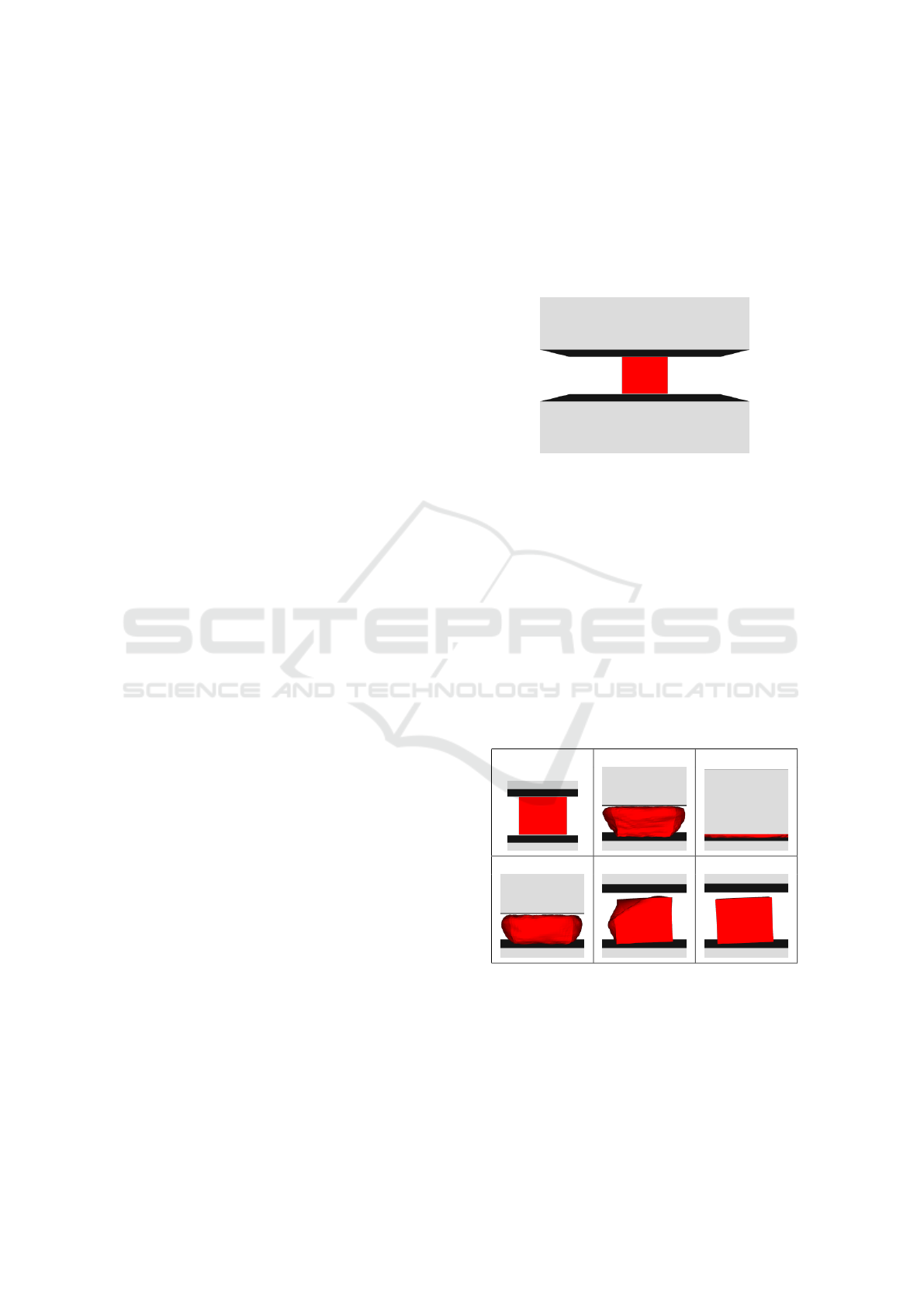
5.1 Artificial Data
To test collision detection and behaviour in extreme
cases, we prepared an artificial dataset, where a box
of 5292 triangles on its surface is squished between
two plates (12 triangles each). The initial setup is vi-
sualized in Fig.1.
Figure 1: Input artificial data.
At first, in one hundred iterations, the top plate
moves to decrease the space between both places.
The distance between plates in 100
th
iteration is 10%
of the original distance in the first iteration. Inverse
movement is then performed between 100
th
and 200
th
iteration, returning the plates to their initial position.
Additional one hundred iterations are used for box
stabilization.
As it can be seen in Fig.2, the box is squished quite
a lot. Despite the fact, it returns to its original shape
in 300
th
iteration (only with slight rotation caused by
asymmetrical triangulation). Even in 200
th
iteration
the results is acceptable, except one corner of the box.
0 50 100
150 200 300
Figure 2: Results in different simulation frames (artificial
data).
5.2 Iliacus
We also tested iliacus muscle, which connects the fe-
mur and pelvic bones from the front side. The bones
and the muscle are visualized in Fig.3. The muscle
HEALTHINF 2020 - 13th International Conference on Health Informatics
220
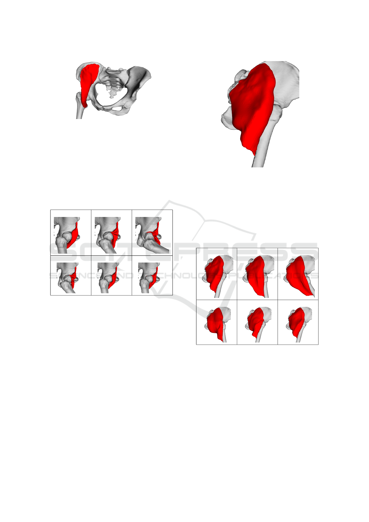
Figure 3: Input iliacus muscle and adjacent bones.
and bones are closed triangular meshes with 13858
and 254442 (42456 for femur) triangles, respectively.
A very similar simulation scenario like in the ar-
tificial data case has been applied to iliacus dataset.
The first hundred iterations are used for hip flexion.
The femur bone rotates one radian during this move-
ment. The second hundred iteration is allocated for
the inverse movement. The last hundred (200
th
-300
th
)
iterations are present to stabilize the muscle.
0 50 100
150 200 300
Figure 4: Results in different simulation frames (Iliacus
muscle data).
The posterior part of the iliacus muscle is pushed
into the joint during the flexion, as it can be seen in
Fig.4. The explanation for this behaviour is as fol-
lows. This part of the mesh is unrealistically arched
towards the joint and, therefore, distance and local
shape constraints tend to move the points of this part
closer to the joint. As the femur and pelvic bones do
not touch, there is a narrow space into which this part
of the mesh can squeeze, and from which it is difficult
to get out. Even though the result is not visually plau-
sible, the quantitative tests (described later) show that
all key factors of the muscle are preserved as much as
possible.
5.3 Gluteus Maximus
Gluteus maximus muscle is attached to the same
bones as iliacus muscle but from the other side. Tri-
Figure 5: Input gluteus maximus muscle and adjacent
bones.
angular mesh of the consits of 19752 triangles. Fig.5
shows how the model looks like.
The muscle undergoes the same movement sce-
nario as iliacus mentioned above. Visualization in 6
important iterations is shown in Fig.6. As we can see,
the result in iteration 300 is nearly the same as in the
first iteration (the original muscle pose).
0 50 100
150 200 300
Figure 6: Results in different simulation frames (gluteus
maximus muscle data).
5.4 Other Muscles
Within this testing procedure, we have tested gluteus
medius and adductor brevis muscles. Both muscles
deform quite realistically, as it can be see in Fig.7 and
Fig.8, where the situation in the maximal hip flexion
(same scenario like in gluteus maximus and iliacus
case) is shown.
Fast and Realistic Approach to Virtual Muscle Deformation
221
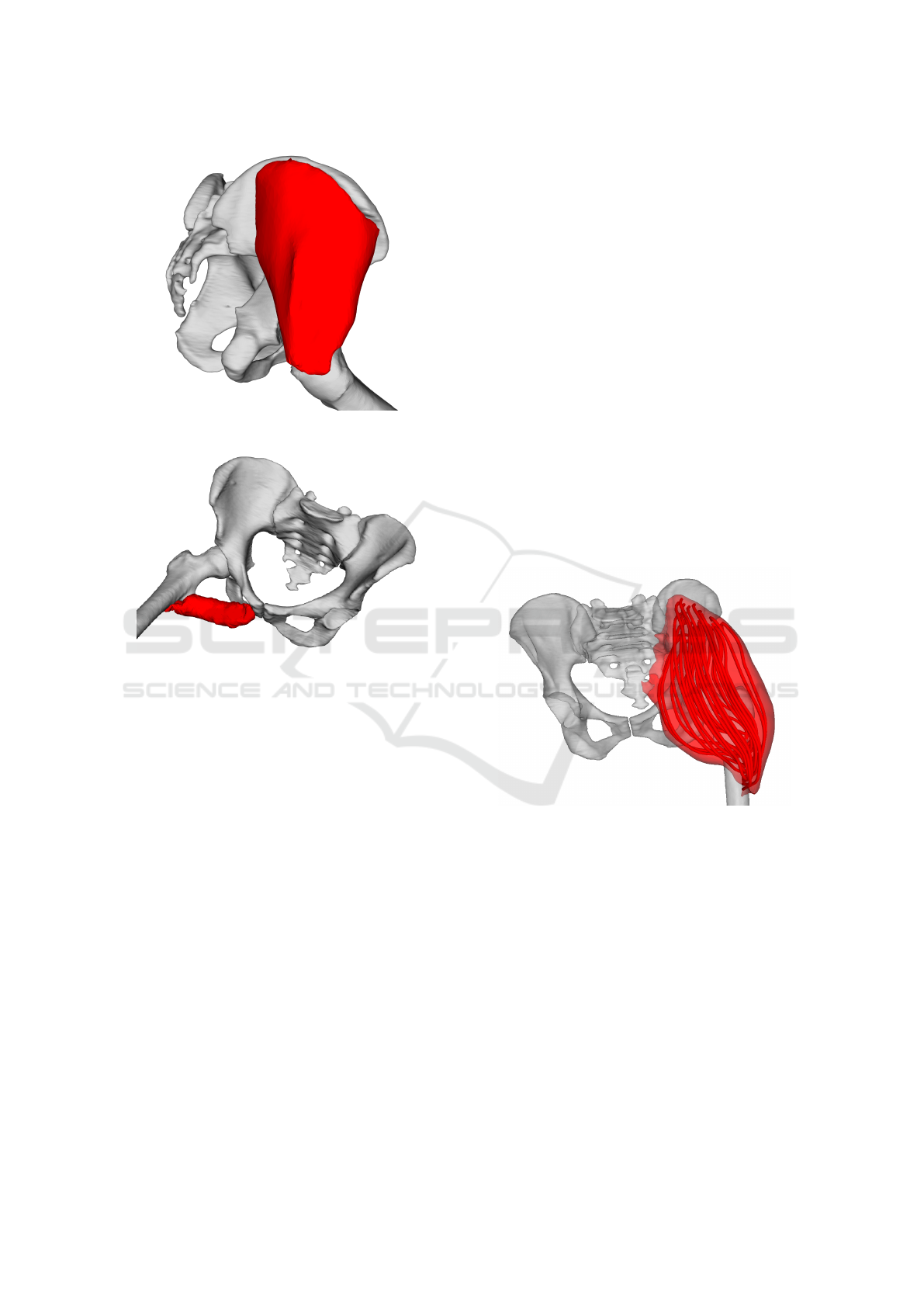
Figure 7: Gluteus medius in maximum flexion position.
Figure 8: Adductor brevis in maximum flexion position.
5.5 Muscle Decomposition
The approach described so far works primarily with
the surface model of a muscle. To calculate the forces
(and other physical properties of the muscle), the
muscle needs to be decomposed into individual fibres.
This can be done using, for example, Kukacka or
CHMD muscle decomposition methods, which were
proposed in (Kohout and Kukacka, 2014) and (Ko-
hout and Cholt, 2017), respectively. In the following
subsections, we briefly describes these methods.
5.5.1 Kukacka Decomposition
The inputs of the Kukacka decomposition method
(Kohout and Kukacka, 2014) are:
• Triangular (and manifold) surface model of the
muscle to decompose,
• Fibre template, giving information about internal
fibre arrangement,
• Attachment areas to adjacent bones (origin and in-
sertion), defined by a set of points lying on the
adjacent bone surface models
Decomposition is then done as follows. Attach-
ment areas are projected from the bone surface onto
the muscle surface to define the parts of the mus-
cle that are subsequently removed. Isocontours are
then computed on the modified muscle model, using
a piece-wise linear scalar field. The scalar field has its
maximum on the insertion boundary vertices, whereas
it has its minimum on the origin boundary vertices.
User can specify how many isocontours are generated
in this process.
Similarly to (Delp, 2005), muscle fibre architec-
ture (template) is represented by a unit 3D space
with arbitrary (user-defined) number of fibres inside
the space. The fibres are represented analytically by
Bezier spline curves. From multiple templates, one is
selected according to the muscle being modelled (de-
pends on if it has parallel or pennate fibres, optionally
on a pennate angle, etc.) and it is mapped one-to-one
on isocontours calculated in the previous step, form-
ing the fibres going through the muscle model. Fi-
nally, noise is eliminated using quadratic smoothing
to make the result more realistic and visually plausi-
ble.
Figure 9: Gluteus maximus decomposed to individual fibres
by Kukacka’s (Kohout and Kukacka, 2014) algorithm.
5.5.2 CHMD Decomposition
A technique by Kohout & Cholt (Kohout and Cholt,
2017) performs a centripetal Catmull-Rom interpo-
lation of the input fibres lying on the surface model
of the muscle, or nearby, to get the fibres inside the
muscle. Their approach can even work with multiple
headed muscles, distributing the fibres automatically
among the heads.
In comparison with Kukacka’s proposed method,
this method needs specification of fibres on the sur-
face, which typically requires some manual effort
because these are not available for the patient but
must be adopted from a cadaveric dataset. On the
HEALTHINF 2020 - 13th International Conference on Health Informatics
222
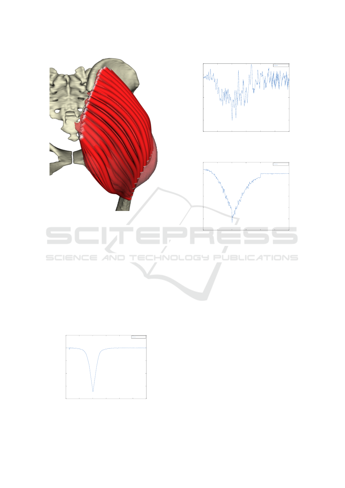
Figure 10: Gluteus maximus decomposed to fibres by
Cholt’s (Kohout and Cholt, 2017) algorithm.
other hand, it can work with multiple headed muscles,
whereas Kukacka’s approach can not.
5.6 Quantitative Tests
To make some exact result, we use quantitative tests.
These tell us how well are constraints satisfied during
simulation.
Volume preservation constraint is tested by deter-
mining ratio between both original and actual vol-
umes. Fig.11 for artificial data, Fig.12 and Fig.13 for
real data respectively, show us the volume preserva-
tion results.
0 50 100 150 200 250 300
0.2
0.4
0.6
0.8
1
1.2
Iteration
Actual/original volume ratio
Volume preservation - Artificial
Volume ratio
Figure 11: Volume preservation of artificial data.
0 50 100 150 200 250 300
0.99
0.992
0.994
0.996
0.998
1
1.002
Iteration
Actual/original volume ratio
Volume preservation - Iliacus
Volume ratio
Figure 12: Volume preservation of iliacus muscle data.
0 50 100 150 200 250 300
0.99
0.992
0.994
0.996
0.998
1
1.002
Iteration
Actual/original volume ratio
Volume preservation - Glut. max.
Volume ratio
Figure 13: Volume preservation of gluteus maximus muscle
data.
As we can see from the results, the volume is well
preserved in both real data (the error is less than 1% in
both cases), on artificial data, there is a nice curve de-
scribing squishing (reducing) box volume during the
simulation and then restoring.
Next measurable property is average edge exten-
sion. At first, we cannot say much about artificial data
(squished box) from the plot on Fig.14. As for the il-
iacus muscle, some edges remain longer than normal
(see Fig.15) because they are stuck in the hip joint. In
the case of gluteus maximus dataset (Fig.16), the first
100 iterations show edge extension during hip flexion
(it is correct behaviour because muscle extends in this
phase) and the second hundred iterations return the
average length extension to almost 1 (i.e., the mus-
cle returns to its original pose correctly). We can also
see that the last 100 iterations are not crucial in this
scenario.
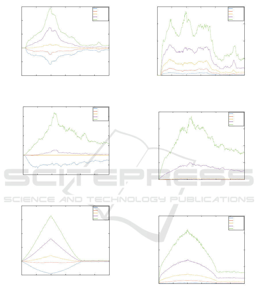
We also tested how well the dihedral angles are
preserved during the simulation. In this paper, the di-
hedral angle is the angle between two adjacent trian-
gles in the muscle triangle mesh. According to plots
in Fig.17, Fig.18 and Fig.19, we can conclude that
there are some pairs of triangles which do not pre-
Fast and Realistic Approach to Virtual Muscle Deformation
223
0 50 100 150 200 250 300
0.6
0.8
1
1.2
1.4
1.6
Iteration
Actual/original edge length
Edge length extension - Artificial
10% quartile
25% quartile
50% quartile
75% quartile
90% quartile
Figure 14: Average edge extension of artificial data.
0 50 100 150 200 250 300
0.96
0.98
1
1.02
1.04
1.06
1.08
1.1
Iteration
Actual/original edge length
Edge length extension - Iliacus
10% quartile
25% quartile
50% quartile
75% quartile
90% quartile
Figure 15: Average edge extension of iliacus muscle data.
0 50 100 150 200 250 300
0.9
1
1.1
1.2
1.3
1.4
Iteration
Actual/original edge length
Edge length extension - Glut. max.
10% quartile
25% quartile
50% quartile
75% quartile
90% quartile
Figure 16: Average edge extension of gluteus maximus
muscle data.
serve its original angle, but most of them do.
5.7 Fibre Length
Last but not least, the lengths of fibres were analyzed.
In the iliacus muscle case, as we can see in Fig.20,
many length curves exhibit two big bumps shortly af-
ter 100
th
iteration. This is caused by the fact that a
0 50 100 150 200 250 300
0
0.2
0.4
0.6
0.8
Iteration
Absolute dihedral angle change [degrees]
Dihedral angle preservation - Artificial
10% quartile
25% quartile
50% quartile
75% quartile
90% quartile
Figure 17: Average absolute dihedral angle change of arti-
ficial data.
0 50 100 150 200 250 300
0
0.05
0.1
0.15
0.2
Iteration
Absolute dihedral angle change [degrees]
Dihedral angle preservation - Iliacus
10% quartile
25% quartile
50% quartile
75% quartile
90% quartile
Figure 18: Average absolute dihedral angle change of ilia-
cus muscle data.
0 50 100 150 200 250 300
0
0.05
0.1
0.15
0.2
Iteration
Absolute dihedral angle change [degrees]
Dihedral angle preservation - Glut. max.
10% quartile
25% quartile
50% quartile
75% quartile
90% quartile
Figure 19: Average absolute dihedral angle change of glu-
teus maximus muscle data.
part of the muscle is stuck in the hip joint (as dis-
cussed previously). Nevertheless, when the bones re-
turn to their initial rest-pose (i.e., after 200 iterations),
the vast majority of fibres restore their original lengths
quite well. Gluteus maximus muscle behaves as ex-
pected – see Fig.21. During the flexion, all lengths
increase; during the extension, they decrease.
HEALTHINF 2020 - 13th International Conference on Health Informatics
224
0 50 100 150 200 250 300
140
160
180
200
220
240
Iteration number
Fibre length [mm]
Fibre lengths - Iliacus
Figure 20: Total length of each individual fibre during sim-
ulation in iliacus muscle.
0 50 100 150 200 250 300
150
200
250
300
350
400
Iteration number
Fibre length [mm]
Fibre lengths - Gluteus maximus
Figure 21: Total length of each individual fibre during sim-
ulation in gluteus maximus muscle.
5.8 Speed
The proposed method was designed to be not only
precise, but mainly, fast. It was implemented in
C++ using VTK toolkit. Its current version is
publicly available at https://github.com/cervenkam/
muscle-deformation-PBD.
All testing scenarios above were measured how
fast each one is. FPS (Frames Per Second) is used
as speed metric in this case.
All tests were performed on Intel
R
Core
TM
i7-
4930K 3.40GHz CPU, Radeon HD 8740 GPU and
WDC WD40EURX-64WRWY0 4TB HDD. Results
are listed on Tab.1.
As it can be seen from the results, FPS strictly de-
pends on number of triangles (Spearman’s ρ = −1).
The more triangles is used, the slower the method is.
Even though the program is mostly unoptimized
and runs sequentially at the moment, the FPS is suffi-
cient for considered purposes in general.
Table 1: FPS of each simulation.
Deforming object Triangle count FPS
Gluteus maximus 19752 33.85
Abductor brevis 17124 35.89
Iliacus 13858 47.21
Gluteus medius 10622 57.12
Artificial box 5292 153.61
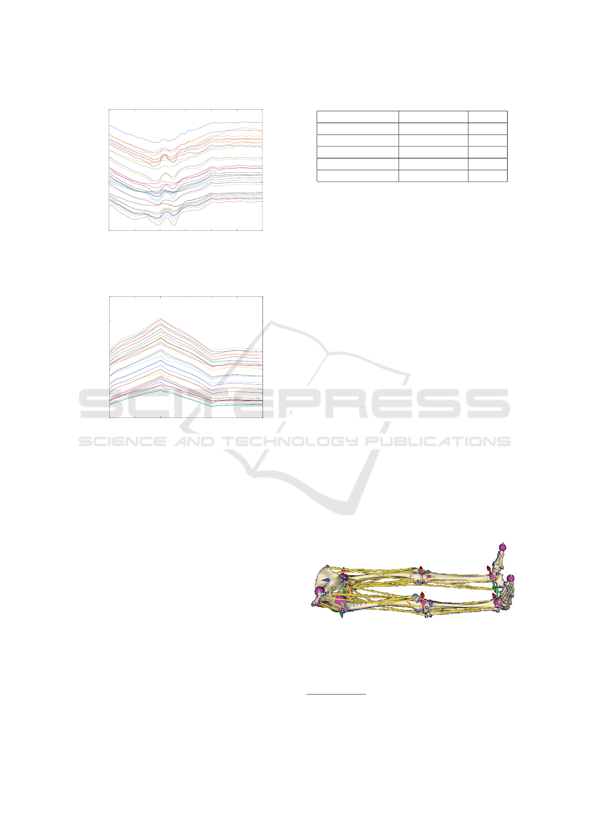
6 DISCUSSION
The most simple approach to muscle deformation
problem is probably to use line segments to approxi-
mate both muscles and tendons. An example is shown
in Fig.22. The coordinates of each end-point of the
corresponding line segments are updated when bone
moves, causing shortening or extending of the line
segments. Various values (e.g., moment arms) can be
consequently calculated from the length of each line.
These models are popular in practice (they are used,
e.g., in AnyBody
1
or OpenSim
2
) because of their sim-
plicity and speed. However, the accuracy of calcula-
tions based on these models is, especially, for com-
plex muscles, e.g., gluteus medius, low (Delp, 2005).
A model can be more precise if we assume more lines
(Valente et al., 2012) per a muscle or if we use more
complex lines wrapping around some kind of para-
metric surfaces (e.g. spheres, cylinders (Audenaert
and Audenaert, 2008), etc.), nonetheless, all of these
are difficult to set up. This may be the reason why
most studies use gait2392 model shipped with Open-
Sim software even though there are no more than
three lines per muscle and these lines penetrate the
bones in some poses. Using our approach, described
in this paper, the user can easily generate hundreds of
lines (i.e., fibres) automatically and impenetrability of
muscles and bones is guaranteed.
Figure 22: Muscle approximation using line segments – yel-
low lines (taken from (Kohout et al., 2013)).
Position-based dynamics (PBD), which is the core
part of our approach, was firstly introduced in (M
¨
uller
et al., 2007) as a computer graphics algorithm. Since
1
https://www.anybodytex.com/software/
2
https://opensim.stanford.edu/
Fast and Realistic Approach to Virtual Muscle Deformation
225

then, it has been further developed (e.g., (Macklin
et al., 2019) proposed recently some speed and ac-
curacy improvements) and has found many (close to)
real-time applications, not only in computer graph-
ics but even in other domains. For example, Kotsalos
et. al. use PBD to model blood cells (Kotsalos et al.,
2019). As far as we know, however, there is no PBD-
based method for muscle modelling even though one
could expect a good compromise between speed and
accuracy from such a method.
A mass-spring system (MSS) is another approach
to consider. Janak et al. use MSS to approxi-
mate muscle (Janak, 2012), showing promising, sim-
ple method with visually plausible results. How-
ever, there are some issues in the approach they pro-
posed. First, to avoid penetration between muscles
and bones, the authors choose a particle-based colli-
sion detection method requiring many particles to get
reasonable results, which, however, causes high time
and memory complexity. Secondly, and more impor-
tantly, the main issue is that muscle volume is not pre-
served during deformation. This could be probably
solved using the approach described in (Hong et al.,
2006), however, it would increase computational time
dramatically. Finally, our experiments show that al-
though this method retains the smooth shape of ili-
acus muscle during flexion, it twists the part of the
muscle close to the insertion. This is because, un-
like our method, the particles are in the entire volume
of the muscle, which results in a model that is much
more rigid, and as anisotropy is not exploited, rigid in
all directions. Our method supports anisotropy, pre-
serves the volume and runs in a fraction of time while
requiring no extra parameter or input in comparison
with this method.
On the contrary to line segment approximation,
finite element method (FEM) is the most complex
method. Well discretized muscle provides a phys-
ically very accurate result (see e.g., (Delp, 2005)).
However, computational complexity is high, mean-
ing the FEM-based methods are unsatisfactorily slow.
Therefore, it is quite impractical for real-time appli-
cation or even clinical assessments. Next issue is a
difficult set up of FEM methods, making them un-
suitable for personalised musculoskeletal method de-
formation. Despite these facts, these methods can be
seen in the movie industry, see e.g. Ziva VFX
3
plu-
gin for Maya, and in muscle physiology research, see
e.g. (Oberhofer et al., 2009) or (Kojic et al., 1998). In
comparison with these methods, our method is quite
simple to set up and runs fast providing the promising
results in most cases.
3
https://zivadynamics.com/
7 CONCLUSION & FUTURE
WORK
The proposed muscle deformation technique is capa-
ble to do fast and relatively accurate simulation. De-
spite problems with muscle trapped in the hip joint,
we believe that a better collision detection can fix the
issue.
Moreover, the method is ready to be included in
OpenSim (a state-of-the-art simulation software) as
a plugin, allowing common users to use the method
more intuitively. Its source code is available at https:
//github.com/cervenkam/muscle-deformation-PBD.
In this paper, we verified the method, but to prove
correctness, the method needs to be validated in real
life. There are some works (e.g. (Modenese et al.,
2018)) providing correct momentum values during
muscle movement, which can be useful for validation.
ACKNOWLEDGMENT
Authors would like to thank their colleagues and stu-
dents for valuable discussion, worthful suggestions
and constructive comments. Authors would like to
thank also anonymous reviewers for their hints and
notes provided.
REFERENCES
Arnold, E., Ward, S., Lieber, R., and Delp, S. (2009). A
model of the lower limb for analysis of human move-
ment. Annals of biomedical engineering, 38:269–79.
Audenaert, A. and Audenaert, E. (2008). Global optimiza-
tion method for combined spherical-cylindrical wrap-
ping in musculoskeletal upper limb modelling. Com-
puter methods and programs in biomedicine, 92:8–19.
Bergmann, G., Deuretzbacher, G., Heller, M., Graichen, F.,
Rohlmann, A., Strauss, J., and Duda, G. (2001). Hip
contact forces and gait patterns from routine activities.
Journal of Biomechanics, 34(7):859 – 871.
Cignoni, P., Callieri, M., Corsini, M., Dellepiane, M.,
Ganovelli, F., and Ranzuglia, G. (2008). Meshlab:
an open-source mesh processing tool. Computing,
1:129–136.
Delp, S. (2005). Three-dimensional representation of com-
plex muscle architectures and geometries 1. Annals
of Biomedical Engineering - ANN BIOMED ENG,
33:1134–1134.
Delp, S. L., Loan, J. P., Hoy, M. G., Zajac, F. E., Topp,
E. L., and Rosen, J. M. (1990). An interactive
graphics-based model of the lower extremity to study
orthopaedic surgical procedures. IEEE Transactions
on Biomedical Engineering, 37(8):757–767.
HEALTHINF 2020 - 13th International Conference on Health Informatics
226

Hong, M., Jung, S., Choi, M.-H., and Welch, S. (2006). Fast
volume preservation for a mass-spring system. IEEE
computer graphics and applications, 26:83–91.
Janak, T. (2012). Fast soft-body models for musculoskele-
tal modelling. Technical Report DCSE/TR-2012-5,
University of West Bohemia, Faculty of Applied Sci-
ences.
Kohout, J. and Cholt, D. (2017). Automatic reconstruc-
tion of the muscle architecture from the superficial
layer fibres data. Computer Methods and Programs
in Biomedicine, 150.
Kohout, J., Clapworthy, G., Zhao, Y., Tao, Y., Gonzalez-
Garcia, G., Dong, F., Wei, H., and Kohoutov
´
a, E.
(2013). Patient-specific fibre-based models of muscle
wrapping. Interface focus, 3:20120062.
Kohout, J. and Kukacka, M. (2014). Real-time modelling of
fibrous muscle. Computer Graphics Forum, 33(8):1–
15.
Kojic, M., Mijailovic, S., and Zdravkovic, N. (1998).
Modelling of muscle behaviour by the finite element
method using hill’s three-element model. Interna-
tional Journal for Numerical Methods in Engineering,
43(5):941–953.
Kotsalos, C., Latt, J., and Chopard, B. (2019). Bridging
the computational gap between mesoscopic and con-
tinuum modeling of red blood cells for fully resolved
blood flow. Journal of Computational Physics, 398.
cited By 0.
Macklin, M., Storey, K., Lu, M., Terdiman, P., Chentanez,
N., Jeschke, S., and M
¨
uller, M. (2019). Small steps in
physics simulation. In Proceedings of the 18th Annual
ACM SIGGRAPH/Eurographics Symposium on Com-
puter Animation, SCA ’19, pages 2:1–2:7, New York,
NY, USA. ACM.
Modenese, L., Montefiori, E., Wang, A., Wesarg, S., Vice-
conti, M., and mazz
`
a, C. (2018). Investigation of the
dependence of joint contact forces on musculotendon
parameters using a codified workflow for image-based
modelling. Journal of Biomechanics.
M
¨
uller, M., Heidelberger, B., Hennix, M., and Ratcliff, J.
(2007). Position based dynamics. Journal of Visual
Communication and Image Representation, 18:109–
118.
Oatis, C. (2013). Kinesiology: The mechanics and path-
omechanics of human movement: Second edition.
Lippincott Williams & Wilkins.
Oberhofer, K., Mithraratne, K., Stott, N. S., and Ander-
son, I. A. (2009). Anatomically-based musculoskele-
tal modeling: prediction and validation of muscle de-
formation during walking. Vis. Comput., 25(9):843–
851.
Shao, X., Liao, E., and Zhang, F. (2017). Improving sph
fluid simulation using position based dynamics. IEEE
Access, PP:1–1.
Valente, G., Martelli, S., Taddei, F., Farinella, G., and
Viceconti, M. (2012). Muscle discretization affects
the loading transferred to bones in lower-limb muscu-
loskeletal models. Proc. Inst. Mech. Eng. H J. Eng.
Med., 226(2):161–169.
Van Sint Jan, S. (2005). Introducing anatomical and physi-
ological accuracy in computerized anthropometry for
increasing the clinical usefulness of modeling sys-
tems. Critical Reviews in Physical and Rehabilitation
Medicine, 17:149–174.
Viceconti, M., Clapworthy, G., and Van Sint Jan, S. (2008).
The virtual physiological human — a european initia-
tive for in silico human modelling —. The journal of
physiological sciences : JPS, 58:441–6.
Wade, S. W., Strader, C., Fitzpatrick, L. A., Anthony, M. S.,
and O’Malley, C. D. (2014). Estimating prevalence of
osteoporosis: examples from industrialized countries.
Archives of Osteoporosis, 9(1):182.
Zhang, J., Fernandez, J., Hislop-Jambrich, J., and Besier,
T. F. (2016). Lower limb estimation from sparse land-
marks using an articulated shape model. Journal of
Biomechanics, 49(16):3875 – 3881.
Fast and Realistic Approach to Virtual Muscle Deformation
227
