
Quantitative Analysis of Facial Paralysis using GMM and Dynamic
Kernels
Nazil Perveen
1 a
, Chalavadi Krishna Mohan
1 b
and Yen Wei Chen
2 c
1
Department of Computer Science and Engineering, IIT Hyderabad, Hyderabad, India
2
College of Information Science and Engineering, Ritsumeikan University, Kusatsu, Shiga, Japan
Keywords:
Facial Paralysis, Spatial and Temporal Features, Gaussian Mixture Model, Dynamic Kernels, Expression
Modeling, Yanagihara Grading Scales.
Abstract:
In this paper, the quantitative assessment for facial paralysis is proposed to detect and measure the different
degrees of facial paralysis. Generally, difficulty in facial muscle movements determines the degree with which
patients are affected by facial paralysis. In the proposed work, the movements of facial muscles are captured
using spatio-temporal features and facial dynamics are learned using large Gaussian mixture model (GMM).
Also, to handle multiple disparities occurred during facial muscle movements, dynamic kernels are used,
which effectively preserve the local structure information while handling the variation across the different de-
gree of facial paralysis. Dynamic kernels are known for handling variable-length data patterns efficiently by
mapping it onto a fixed length pattern or by the selection of a set of discriminative virtual features using mul-
tiple GMM statistics. These kernel representations are then classified using a support vector machine (SVM)
for the final assessment. To show the efficacy of the proposed approach, we collected the video database of
39 facially paralyzed patients of different ages group, gender, and from multiple angles (views) for robust
assessment of the different degrees of facial paralysis. We employ and compare the trade-off between accu-
racy and computational loads for three different categories of the dynamic kernels, namely, explicit mapping
based, probability-based, and matching based dynamic kernel. We have shown that the matching based kernel,
which is very low in computational loads achieves better classification performance of 81.5% than the existing
methods. Also, with the higher-order statistics, the probability kernel involves more communication overhead
but gives significantly high classification performance of 92.46% than state-of-the-art methods.
1 INTRODUCTION
Facial paralysis is the facial nerve paralysis, which
occurs due to temporary or permanent damage to the
facial nerve. There are multiple reasons like surgi-
cal, neurological, viral infections, injuries, etc., which
causes damage to the facial nerve. Due to the damage
in the facial nerve, there is loss in the movement of the
facial muscles, which restrain the patients to pose nor-
mal facial actions like smiling, closing of eyes, clos-
ing of the mouth, etc. Facial paralysis affect the pa-
tient face either on half or both sides.
To detect the level and intensity of the effect
caused by the facial paralysis to the patients face, mul-
tiple diagnoses are required by the clinicians. Most
a
https://orcid.org/0000-0001-8522-7068
b
https://orcid.org/0000-0002-7316-0836
c
https://orcid.org/0000-0002-5952-0188
of them involve subjective assessments like assign-
ing of grading score to the patient face based on cer-
tain facial expressions. The Yanagihara grading scale
by Hato et al. (2014) and House-Brackmann (HB)
grading scales by House and Brackmann (1985) are
the two mostly used subjective grading scores for
evaluating the facial paralysis and its effects. Due
to the easier interpretation of the grading levels and
the formation of the facial simple expression Satoh
et al. (2000), Yanagihara is the widely used tech-
niques in detecting different levels of facial paraly-
sis. There are 10 expressions in Yanagihara grad-
ing scale like rest videos (EP0), raising of eyebrows
(EP1), closure of eye gently (EP2), closure of eye
tightly (EP3), closure of paralyzed eye (EP4), wrin-
kle nose (EP5), puff out cheeks (EP6), toothy move-
ment (EP7), whistling movement (EP8), and under lip
turn down (EP9). Also, there are two different levels
of the grading scales using Yanagihara grading rules,
Perveen, N., Mohan, C. and Chen, Y.
Quantitative Analysis of Facial Paralysis using GMM and Dynamic Kernels.
DOI: 10.5220/0009104801730184
In Proceedings of the 15th International Joint Conference on Computer Vision, Imaging and Computer Graphics Theory and Applications (VISIGRAPP 2020) - Volume 5: VISAPP, pages
173-184
ISBN: 978-989-758-402-2; ISSN: 2184-4321
Copyright
c
2022 by SCITEPRESS – Science and Technology Publications, Lda. All rights reserved
173

i.e, 5-scores, and 3-scores grading scales. In 5-scores
grading scales, the listed expression posed by the pa-
tient is graded from score-0 to score-4, where score-0
denotes high-level of facial paralysis, score-1 denotes
almost facial paralysis, score-2 represents moderate,
score-3 represents slight facial paralysis and score-
4 denotes no facial paralysis. Similarly, in 3-scores
grading scales, the listed expression posed by the pa-
tient is graded from score-0 to score-2, where score-0
denotes high-level of facial paralysis and score-2 de-
notes low-level of facial paralysis (or no paralysis),
respectively.
Although subjective assessments are widely used
techniques but it highly depends on the expert’s opin-
ion of assigning grades while examining the patients
during facial expressions formation. This motivates
our research to develop a generalized model for the
quantitative assessments of the facial paralysis using
different dynamic kernels. Kernels effectively pre-
served the local structure and also able to handle large
variation globally. Thus, in the proposed approach
once the local attributes are captured implicitly by
the components of universal GMM, the kernels are
learned for the better representation of the video both,
locally and globally. Also, the video data mostly con-
tains a variable length sequence of the local feature
vector, therefore to handle the variability in the se-
quence of local features extracted from the videos,
dynamic kernels are used Dileep and Sekhar (2014).
The paper is organized as follows. In Section 2,
we discuss the previous work done for the quantitative
assessment of facial paralysis. Section 3 describes
the proposed quantitative assessment method in de-
tail. Experimental results are discussed in Section 4
to show the efficacy of the proposed approach. Sec-
tion 5 concludes the work with future directions.
2 RELATED WORK
NGO et al. (2016) proposed the quantitative assess-
ment of the facial paralysis using 2D features. These
2D features were novel and robust spatio-temporal
features, which were computed frame-wise. Initially,
face was detected in the given frame using the Ad-
aBoost algorithm and then landmarks points were de-
tected. The facial landmark points were detected by
computing region of interest (ROI) using the perpen-
dicularity of inter-pupil distance with vertical face
mid line. Once the ROI area was selected the land-
mark points were placed and tracked throughout the
frames. The spatio-temporal features were extracted
using the tracked landmark points, which were then
classified using support vector machine (SVM) for
finding a different level of facial paralysis. The av-
erage accuracy achieved by this method is approxi-
mately 70% for only three categories of expressions
for 5-scoring levels.
He et al. (2009), proposes the novel block process-
ing techniques to capture the appearance information
at different resolutions. They use local binary pat-
tern (LBP) to extract appearance features from the
apex frame (i.e the frame in which facial expression is
highly active) at multiple block levels and at different
resolutions, which is known as multi-resolution LBP
(MLBP). These blocks were centered over the facial
regions like eyebrows, eyes, nose, and mouth. They
also, extracted motion information by tracking the fa-
cial muscle movement in the horizontal (x-axis) and
vertical (y-axis) direction. Once the feature from dif-
ferent regions is extracted they compare the symme-
try between normal facial regions with the paralyzed
facial region using resistor-average distance (RAD).
Finally, they use a support vector machine for the fi-
nal assessment and score prediction based on RAD.
They evaluate their model with the House-Brackmann
(HB) grading scale on the self-collected and anno-
tated database. They use four expressions with a 5-
score grading scale to achieve average classification
rate of 86.6%.
Liu et al. (2015) propose the thermal imaging
model for learning the facial paralysis effect. The
proposed approach demonstrate the change in facial
nerve functions, when the facial temperature changes.
The medical infrared thermal imager made of liquid
nitrogen was used for facial temperature distribution
acquisition. For collecting the infrared thermal im-
age dataset, patients should not drink and must sit for
20 minutes prior to adapt the room temperature be-
fore experiments start. Using the features like tem-
perature distribution, area ratio, and temperature dif-
ference over the region of interest of normal and para-
lyzed facial area, they classify the different level of fa-
cial paralysis. For classification, K-nearest neighbor
classifier (K-NN), support vector machines (SVM),
and radial basis function neural network (RBFNN)
was used. They evaluate their model for four expres-
sions with an average accuracy of 94% with RBFNN
classifier.
Banks et al. (2015) developed the offline applica-
tion named eFace for detection of the unilateral facial
paralysis. The video of the patient with posing list of
facial expressions was recorded and fed into the eFace
for comparing the normal and affected side. Differ-
ent score to capture disfigurement severity was calcu-
lated like static scores, dynamic scores, and synkine-
sis score. Based on the computed scores the grading
from 1 to 100 is provided where 1 denotes high dis-
VISAPP 2020 - 15th International Conference on Computer Vision Theory and Applications
174
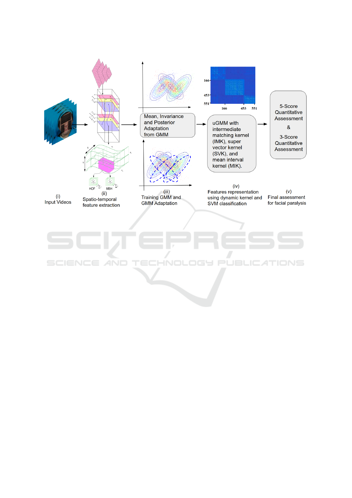
Figure 1: Block diagram of the proposed approach, which comprises of the following steps.
figurement severity and 100 denotes least or no dis-
figurement severity. The evaluation was done on a
self-collected database of 25 subjects under expert su-
pervisions.
Ngo et al. (2016) proposed the objective evalua-
tion of the facial paralysis using 3D features. The
facial landmark points were evaluated from the first
frame, which was tracked throughout the frames for
the given video. These landmarks points were then
used to calculate asymmetrically and movement fea-
tures in the 3-D space for capturing and comparing
the facial muscle movement between normal and par-
alyzed side of the face. This objective evaluation of
facial paralysis achieves an average recognition rate
of 66.475% for the four prominent expressions, i.e for
EP1, EP3, EP5, and EP7, respectively, for 5-scoring
levels.
Recently, Guo et al. (2017) proposed the deep neu-
ral network model for classifying the severity of the
facial paralysis. They use Google LeNet model for
the self-collected private database from 104 subjects.
They achieved the performance of 91.25% for four
expressions with a 5-score House-Brackmann (HB)
grading scale.
Thus, the related works mentioned above is highly
subjective and most of the approaches are based on
asymmetric features. Faces considered in the above
approaches are mostly frontal with patient posing
very few active expressions like opening and clos-
ing of eyes, mouth, etc. This motivates us to develop
the generalized model for predicting and classifying
different levels of facial paralysis by considering all
listed expressions in the literature. The following are
the major contribution of the paper:
1. The proposed approach train a large GMM with
seven views and multiple subjects to learn view
and subject invariant attributes from the videos for
the better assessments.
2. The proposed approach introduces dynamic ker-
nels, which handles the variation across various
facial muscle movements and effectively preserve
the local dynamic structure to distinguish the dif-
ferent degree level of facial paralysis.
3. The proposed approach, model all the 10 expres-
sions mentioned in the Yanagihara grading system
with all available scores i.e. 5-scores and 3-score
grading scales for effective assessment.
Thus, the propose approach address the limita-
tions of the existing work for better quantitative as-
sessment of facial paralysis. The next section de-
scribes the proposed approach in details.
3 PROPOSED APPROACH
The block diagram of the proposed approach is shown
in Figure 1. Initially, face in the collected input videos
is aligned using facial landmark points to remove un-
wanted background information. The aligned faces
Quantitative Analysis of Facial Paralysis using GMM and Dynamic Kernels
175

are then tracked for spatial and temporal feature ex-
traction. These features are then used for training
large Gaussian mixture model (GMM), which is then
used to compute the statistics of GMM for design-
ing of the dynamic kernel for quantitative assessment
of the facial paralysis. The details of the proposed
methodology are given as follows.
3.1 Data Pre-processing and Feature
Extraction
From the aligned face video, two descriptors, namely,
the histogram of optical flow (HOF) and motion
boundary histogram (MBH) features are evaluated us-
ing dense trajectories Wang et al. (2015) as shown in
Figure 1-part (ii). Initially, the dense trajectory fea-
ture points are computed at 8 different spatial scales.
In each scale, the feature points are densely sampled
on a grid spaced by W = 5 pixels. Further, each fea-
ture points are tracked till the next frame by using me-
dian filtering in the dense optical flow field. The tra-
jectories computed are tended to drift from their ini-
tial location if tracked for the longer period, thus, to
avoid the drifting issue the frame length for tracking
is fixed to t = 15 frames.
Further, the local descriptors are computed around
the interest points in 3D video volume, as it is always
the effective way of capturing the motion information.
The size of the video volume considered is P ×P pix-
els, where P = 32. To ensure the dynamic structure of
the video the volume is further subdivided into spatio-
temporal grid of g
h
×g
w
×g
t
, where g
h
= 2, g
w
= 2,
and g
t
= 3 are height, width, and temporal segment
lengths. Once, the HOF and MBH descriptors are
computed from each spatio-temporal grid, it is quan-
tized into 9 and 8 bins, respectively, and normalized
using RootSIFT method as mentioned in Wang et al.
(2015).
The size of the HOF descriptors obtained is of
108 dimensions (i.e., 2 ×2 ×3 ×9). Also, the size of
MBH descriptors obtained by computing the descrip-
tors from horizontal and vertical components of the
optical flow, i.e MBH in x and y direction are of 192
dimensions (i.e. 96 dimensions for each direction).
The reason for using the above mention dense tra-
jectory, i.e., HOF and MBH descriptors are, all the
trajectories in the given video does not contain useful
information like trajectories cause due to large, sud-
den, and constant camera motions. Therefore these
trajectories are required to remove so to retain only
the essential foreground trajectories caused by the fa-
cial movements. The removal of such trajectories is
efficiently done by the improved dense trajectories,
which are far efficient than commonly used features
like HOG3D, 3DSIFT, and LBP-TOP, etc, that are
usually computed in a 3D video volume around in-
terest points, which usually ignores the fundamental
dynamic structures in the video Wang et al. (2015).
3.2 Training of a Gaussian Mixture
Model (GMM)
The features obtained from different views and sub-
jects from the videos are extracted to train the
large Gaussian mixture model (GMM). The GMM is
trained for multiple components q = 1, 2, ··· , Q in or-
der to capture different facial movement attribute in
various Q components. Given a video V, the set of
local features are represented as v
1
, v
2
, ··· , v
N
, where
N is the total number of local features for the given V .
The likelihood of the particular feature v
n
generated
from the GMM model is given by
p(v
n
) =
Q
∑
q=1
w
q
N (v
n
|µ
q
, σ
q
), (1)
where µ
q
, σ
q
represents mean and covariance for
each GMM component q, respectively. Further, w
q
represents GMM mixture weights, which should sat-
isfy the constraint
∑
Q
q=1
w
q
= 1. Once the GMM is
trained, the probabilistic alignment of each feature
vector v
n
with respect to the qth component of the
GMM model is evaluated using as follows
p(q|v
n
) =
w
q
p(v
n
|q)
∑
Q
q=1
w
q
p(v
n
|q)
, (2)
where p(v
n
|q) is the likelihood of a feature v
n
gen-
erated from a component q. Using the different pa-
rameters of the GMM, multiple dynamic kernel-based
representations are generated, which will efficiently
represent the given video. The next subsections de-
tailed the formulation of the dynamic kernels.
3.3 Dynamic Kernels
The selection of kernel function plays important role
in the performance of kernel methods. For static pat-
terns, several kernel functions are designed in past
decades The kernels designed for the varying length
patterns are known as dynamic kernels. Dynamic ker-
nels are either formed by converting variable length
patterns to static patterns or by designing new ker-
nel functions. In this sub-section, we present different
dynamic kernels, which effectively preserve local and
global information, respectively, for better represen-
tation of the given sample.
VISAPP 2020 - 15th International Conference on Computer Vision Theory and Applications
176

3.3.1 Explicit Mapping based Dynamic Kernel
In the explicit mapping dynamic kernel, the set
of variable length local feature representations are
mapped onto fixed dimensional feature representation
in the kernel space by GMM based likelihood. The
Fisher kernel (FK) used for the proposed approach
maps the set of variable length local features onto
the fixed dimensional Fisher score. The Fisher score
is computed by evaluating the first derivative of log-
likelihood for mean, covariance, and weight vector
using Equation 2 given by
ψ
(µ)
q
(V) =
N
∑
n=1
p(q|v
n
)m
nq
, (3)
ψ
(σ)
q
(V) =
1
2
N
∑
n=1
p(q|v
n
)[−u
q
+ h
nq
]
!
, (4)
ψ
(w)
q
(V) =
N
∑
n=1
p(q|v
n
)
1
w
q
−
p(q
1
|v
n
)
w
1
p(q|v
n
)
. (5)
where m
nq
=
∑
−1
q
(v
n
−µ
q
), u
q
= Σ
−1
q
and h
nq
=
m
n1q
m
T
nq
, m
n2q
m
T
nq
, ··· , m
ndq
m
T
nq
. For any d × d
matrix A with a
i j
, i, j = 1, 2, ··· , d as its elements,
vec(A) = [a
11
, a
12
, ··· , a
dd
]
T
.
The first-order derivative or the gradient of the
log-likelihood computed above represent the direc-
tions in which the parameters, namely, µ, Σ, and w
should be updated for the best fit of the model. We in-
fer that the deviations that occurred, during the facial
movements of particular expressions are captured by
these gradients. The fixed dimensional feature vector
known as the Fisher score vector is then computed by
stacking all the gradients from Equation 3, 4, and 5
given by
Φ
q
(V) =
h
ψ
(µ)
q
(V)
T
, ψ
(σ)
q
(V)
T
, ψ
(w)
q
(V)
T
i
T
. (6)
The Fisher score vector for all the Q components
of the GMM is given by
Φ
s
(V) =
Φ
1
(V)
T
Φ
2
(V)
T
Φ
Q
(V)
T
T
. (7)
The Fisher score vector captures the similarities
across two samples, thus the kernel function for com-
paring two samples V
x
and V
y
, with given local fea-
tures is computed by
K(V
x
, V
y
) = Φ
s
(V
x
)
T
F
−1
Φ
s
(V
y
), (8)
Where I is knows as Fisher information matrix
given by
I =
1
D
D
∑
d=1
Φ
s
(V
d
)Φ
s
(V
d
)
T
. (9)
The Fisher information matrix captures the variabil-
ity’s in the facial movement across the two samples.
Thus both local and global information is captured
using Fisher score and Fisher information matrix in
Fisher kernel computation. However, the computation
complexity for the Fisher kernel is highly intensive.
The computation of gradient for mean, covariance,
and weight matrix involves Q×(N
p
+N
r
), each. Then
the computation of the Fisher information matrix in-
volves D ×d
2
s
+ D computations, where D is the total
number of training examples. Similarly, the Fisher
score vector requires d
2
s
+ d
s
computations, where d
s
is the dimension of the Fisher score vector. Thus, the
total computation complexity of the Fisher kernel is
given as O(QN +Dd
2
s
+D +d
2
s
+d
s
) as shown in Ta-
ble 1.
3.3.2 Probability based Dynamic Kernel
In probability-based dynamic kernels, the set of vari-
able length local feature representations are mapped
onto fixed dimensional feature representation in the
kernel space by comparing the probability distribu-
tions of the local feature vectors. Initially, the maxi-
mum aposteriori (MAP) adaptation of means and co-
variances of GMM for each clip is given by
µ
q
(V) = αF
q
(V) + (1 −α)µ
q
. (10a)
and
σ
q
(V) = αS
q
(V) + (1 −α)σ
q
. (10b)
where F
q
(V) is the first-order and S
c
(V) is the
second-order Baum-Welch statistics for a clip V, re-
spectively, which is calculated as
F
q
(V) =
1
n
q
(V)
N
∑
n=1
p(q|v
n
)v
n
(11a)
and
S
q
(V) = diag
N
∑
n=1
p(q|v
n
)v
n
v
T
n
!
, (11b)
respectively.
The adapted mean and covariance from each
GMM component depend on the posterior probabili-
ties of the GMM given for each sample. Therefore,
if the posterior probability is high then higher will
be the correlations among the facial movements cap-
tured in the GMM components. This shows that the
adapted mean and covariance for each GMM mixture
will have a higher impact than the full GMM model
means and covariances. Thus, the adapted means
from Equation 10a, for sample V is given by
ψ
q
(V) =
√
w
q
σ
−
1
2
q
µ
q
(V)
T
. (12)
Quantitative Analysis of Facial Paralysis using GMM and Dynamic Kernels
177

Table 1: Statistics of the collected database score-wise in 3-score grading scales.
Kernels Number of computations Computational Complexity
Fisher Kernel
(FK)
Gradient vector
computation
3 ×Q ×(N
p
+ N
r
)
O(QN + Dd
2
s
+ D + d
2
s
+ d
s
)
Fisher
information
matrix
D ×d
2
s
+ D
Kernel
computation
d
2
s
+ d
s
Intermediate
matching
kernel
(IMK)
Posterior
probability
computation
Q ×(N
p
+ N
r
)
O(QN)
Comparisons to
select features
Q ×(N
p
+ N
r
)
Base kernel
Computation
Q
GMM
supervector
kernel
(GMM-SVK)
Mean
adaptation
Q ×(N
p
+ N
r
)
O(QN + Qd
2
l
+ d
2
s
)
Supervector
computation
Q ×(d
2
l
+ 1)
Kernel
computation
d
2
s
GMM
mean
interval
kernel
(GMM-MIK)
Mean
adaptation
Q ×(N
p
+ N
r
)
O(QN + Qd
2
l
+ Qd
l
+ Q
2
d
2
s
)
Covariance
adaptation
Q ×(N
p
+ N
r
)
Supervector
computation
Q ×(d
2
l
+ d
l
)
Kernel
computation
d
2
s
By stacking the GMM vector for each
component, a Qd × 1 dimensional super-
vector is obtained, which is known as
GMM supervector (GMM-SV) represented as
S
svk
(V) = [ψ
1
(V)
T
, ψ
2
(V)
T
, ··· , ψ
Q
(V)
T
]
T
.
The GMM-SV used for comparing the similarity
across two samples, namely, V
x
and V
y
by construct-
ing GMM supervector kernel (GMM-SVK), which is
given by
K
svk
(V
x
, V
y
) = S
svk
(V
x
)
T
S
svk
(V
y
). (13)
The GMM-SVK kernel formed above only uti-
lizes the first-order adaptations of the samples for
each GMM components. Thus, the second-order
statistics, i.e., covariance adaptations is also in-
volved in constructing fixed-length representation
from variable-length patterns is given by
ψ
q
(V) =
σ
q
(V) −σ
q
2
!
−
1
2
µ
q
(V) −µ
q
. (14)
Combining the GMM mean interval supervector
(GMM-GMI) for each component is computed as
S
mik
(V) = [ψ
1
(V)
T
, ψ
2
(V)
T
, ··· , ψ
Q
(V)
T
]
T
.
Thus, to compare the similarity across the two
samples V
x
and V
y
, the kernel formation is performed
using GMM-GMI kernel also known as GMM mean
interval kernel (GMM-MIK) given by
K
mik
(V
x
, V
y
) = S
mik
(V
x
)
T
S
mik
(V
y
). (15)
The fixed-length representation formed by using
the posterior probabilities in the kernel space is a
high dimensional vector, which involves Q ×(N
p
+
N
r
) computations for mean adaptation and 2 ×Q ×
(N
p
+ N
r
) for mean and covariance adaptations, re-
spectively. And the kernel computation required
Q ×(d
2
l
+ 1) and d
2
s
, where d
l
is the dimension of
local feature vector. The total computational com-
plexities of GMM-SVK and GMM-MIK kernels are
O(QN +Qd
2
l
+d
2
s
) and O(QN +Qd
2
l
+Qd
l
+Q
2
d
2
s
),
respectively as shown in Table 1.
3.3.3 Matching based Dynamic Kernel
The kernels mentioned above are mentioned based
on the mapping of variable-length feature representa-
VISAPP 2020 - 15th International Conference on Computer Vision Theory and Applications
178

Figure 2: Illustration of the facial paralysis patients posing 10 different expressions under expert supervision. Black patches
are imposed to hid the identity of the patient (best viewed in color).
tions to fixed-length feature representations. This sec-
tion introduces the alternative approach for designing
of the new kernel for handling variable-length data,
known as matching based dynamic kernels. Various
matching based dynamic kernels are proposed in the
literature like summation kernel (SK), matching ker-
nel (MK), etc. However, these kernels are either com-
putationally intensive or not proved to be the Mercer’s
kernel. So, an intermediate matching kernel (IMK) is
formulated by matching a set of local feature vectors
by closest virtual feature vectors obtained using the
training data of all classes. Let Z = {z
1
, z
2
, ··· , z
Q
}
be the virtual feature vectors. Then, the feature vec-
tors v
∗
xq
and v
∗
yq
in V
x
and V
y
, respectively, that are
nearest to q
th
virtual feature vector z
q
is determined
as
v
∗
xq
= argmin
v∈V
x
D(v, z
q
) and v
∗
yq
= argmin
v∈V
y
D(v, z
q
),
(16)
where D(., .) is a distance function, which mea-
sures the distance of a feature vector V
x
or V
y
to the
closest feature vector in Z. We hypothesize that the
distance function aid in finding the closest facial mus-
cle movement learned from the clip to one, which is
captured by GMM components. Once the closest fea-
ture vector is selected, the base kernel will be given
by
K
imk
(V
x
, V
y
) =
Q
∑
q=1
k(v
xq
, v
yq
). (17)
In the proposed approach, the GMM parameters
like mean, covariance, and weight are used as a set of
virtual feature vectors. And, the distance or closeness
measure is computed by using the posterior probabil-
ity of the GMM component generating the feature de-
scribed in Equation 2. Thus, the local feature vectors
close to the virtual feature vector for the given q is
v∗
xq
and v∗
yq
for clips V
x
and V
y
, respectively, which
is computed as
v
∗
xq
= argmax
v∈V
x
p(q|v) and v
∗
yq
= argmax
v∈V
y
p(q|v). (18)
The computational complexity of IMK is very low
compared to other mentioned dynamic kernels de-
fined as (i) Q×(N
p
+ N
r
) comparisons for selection of
closest feature vector, (ii) Q ×(N
p
+ N
r
) required for
posterior probability computations, and (iii) Q base
kernel computations. Thus the total computational
complexity of IMK is given by O(QN) where N is
the set of local feature vector as shown in Table 1.
For classification, support vector machine (SVM)
is built for each dynamic kernel. The SVM is a two-
class classifier, For D training samples can be repre-
sented as (V
d
, y
d
)
D
d=1
, where y
d
represents the label
information of the particular class, then discriminant
function for SVM is given by,
f (V ) =
D
∑
d=1
α
∗
d
y
d
K
DK
(V, V
d
) + b
∗
(19)
where D
s
be the number of support vectors, α
∗
is
the optimal values of the Lagrangian coefficient and
b
∗
is the optimal bias. The sign value of the function
f decides the class of V . We use a one-against rest
approach with 10 fold cross-validation to discriminate
the sample of the particular class with all the other
classes.
4 EXPERIMENTAL RESULTS
In this section, we describes about the facial paralysis
dataset in detail. Also, we analyse different types of
dynamic kernels representations for better quantita-
tive assessments. We compare the proposed approach
with existing state of the art approaches and in last
we discuss the efficacy of the proposed approach with
some ablations study.
4.1 Dataset Collection and Annotation
Protocol
To show the efficacy of the proposed approach we
collected the video dataset of the facially paralyzed
Quantitative Analysis of Facial Paralysis using GMM and Dynamic Kernels
179
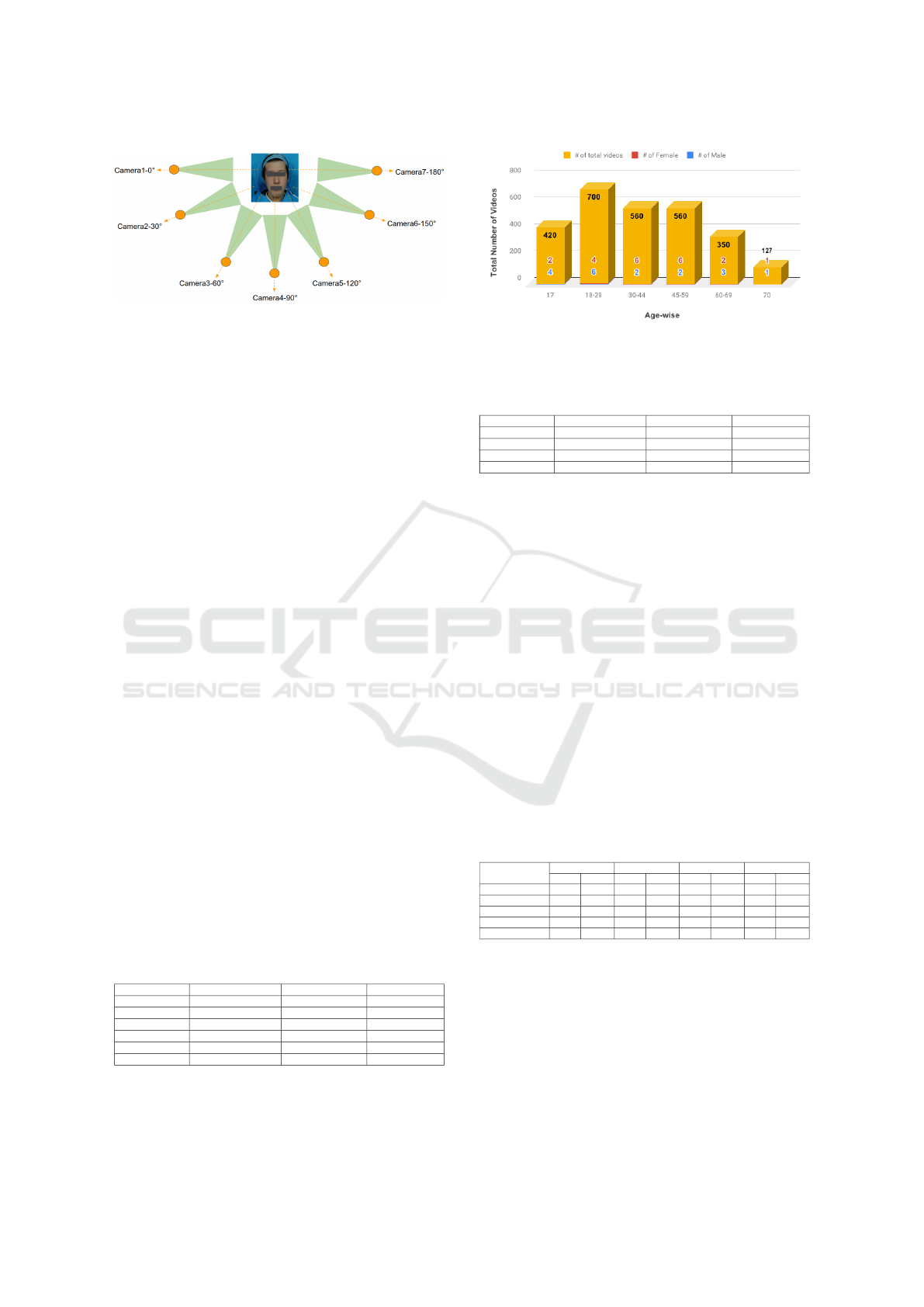
Figure 3: Camera position during the video recording of the
facially paralyzed patients, black patches are added to hide
the identity of the patient (best viewed in color).
patients under 3 expert supervision. The patients
concerned are taken in advance for the collection of
videos. Multiple subjects of various age group, gen-
der, races, etc, are collected. Also, the video recorded
is captured from seven different angle views by plac-
ing multiple cameras at different angle setting of +/-
30
◦
as shown in Figure 3. The main objective of col-
lecting subject and view-invariant videos of the pa-
tients is to develop an accurate and generalized model
for the quantitative assessment of facial paralysis.
The total number of video samples collected for the
experiments is 2717 from 39 subjects. These 39 sub-
jects are of different age starting from 17 years to 70
years, the detailed statistics of the dataset age-wise
and gender-wise is shown in Figure 4. During captur-
ing the patient videos, patients are asked to perform
the 10 expressions given on Figure 2 and also subjec-
tive assessments using Yanagihara grading scale un-
der 3 experts supervision are computed for ground
truth evaluation. The experts also grade the expres-
sions posed by the patients from score-0 to score-5.
As already mention, the grading provided by the ex-
perts are highly subjective, thus, for the ground truth
of the proposed model, we took 2 best subjective ex-
pert opinions out of 3 experts. Based on the subjective
assessments we divided the whole dataset into 2166
training videos and 551 testing videos for score-0 to
score-5 as shown in Table 2 and for score-0 to score-2
as shown in Table 3. Also, the testing video subjects
are not at all present in the training set in any condi-
tions during experimentation.
Table 2: Statistics of the collected database score-wise in
5-score grading scales.
Grading scores # of training videos # of testing videos # of total videos
Score 0 166 62 228
Score 1 322 104 426
Score 2 600 147 747
Score 3 539 140 679
Score 4 539 98 637
Total videos 2166 551 2717
Figure 4: Statistics of the data collected age-wise and
gender-wise (best viewed in color).
Table 3: Statistics of the collected database score-wise in
3-score grading scales.
Grading scores # of training videos # of testing videos # of total videos
Score 0 488 166 655
Score 1 1139 287 1426
Score 2 539 98 637
Total videos 2166 551 2717
4.2 Analysis of the Dynamic Kernels for
Quantitative Assessment of Facial
Paralysis
The classification performance of various dynamic
kernel like Fisher kernel (FK), intermediate matching
kernel (IMK), supervector kernel (SVK), and mean
interval kernel (MIK) using different GMM compo-
nents, namely 32, 64, 128, 256, and 512 is shown
in Table 4 for 5-class grading score. The spatio-
temporal facial features, namely, histogram of optical
flow (HOF) and motion boundary histogram (MBH)
are trained using GMM and classified using kernel-
based support vector machine (SVM) Cortes and Vap-
nik (1995). It can be observed that the best perfor-
Table 4: Classification performance (%) of FK, IMK, SVK,
and MIK on different GMM components for 5-class grading
score.
# of
components
FK IMK SVK MIK
HOF MBH HOF MBH HOF MBH HOF MBH
32 37.3 40.1 67.1 70.5 68.8 74.1 70.5 75.2
64 43.6 44.5 72.3 73 69.7 76.2 72 75.8
128 45.5 45.5 74.1 75.8 71.4 77.3 73 78.6
256 47.9 48.6 76.6 77.9 78.4 82.2 86.5 90.7
512 46.8 47.9 76.2 76.2 72.3 78.4 81.5 87.1
mance kernels are probability-based kernels, namely,
support vector kernel (SVK) and mean interval kernel
(MIK) as it captures the first-order and second-order
statistics of the learned GMM model. Also, it can
be observed that increasing the number of mixtures
in GMM increases the better generalization capability
of the model, however, it cannot be increased beyond
256 due to increase in demand of the local feature in-
formation, which cannot be addresses due to the lim-
VISAPP 2020 - 15th International Conference on Computer Vision Theory and Applications
180

(a) 5-class grading score (b) 3-class grading score
Figure 5: Confusion matrix of MBH feature vector using GMM-MIK dynamic kernel with SVM for 256 components (best
viewed in color).
ited size of the dataset.
The confusion matrix for 5-class grading score is
given in Figure 5 (a), it can be observed that the mis-
classified samples are mostly present in the neighbor-
ing class, due to which we combined the score-0 class
examples with score-1 class examples and the score-2
class examples with score-3 class examples. Follow-
ing the previous work Ngo et al. (2016), NGO et al.
(2016), and Wachtman et al. (2002), we reduce the
number of classes from 5-class grading score to 3-
class grading to facilitate the comparison of the pro-
posed work with the state of the art approaches. The
classification performance of the above fusion i.e. for
3-class grading scores are shown in Table 5 and con-
fusion matrices for the best performances are shown
in Figure 6.
Table 5: Classification performance (%) of FK, IMK, SVK,
and MIK on different GMM components for 3-class grading
score.
# of
components
FK IMK SVK MIK
HOFMBHHOFMBHHOFMBHHOFMBH
32 52.6 53.8 68.8 71.4 71.4 72.3 85.9 87.2
64 53.7 55.2 70.5 75.8 76.8 79.2 86.9 89
128 55.2 58.2 73.2 76.2 78.8 79.9 88.9 90.8
256 62.3 63.2 78.4 81.5 82.4 84.1 90.2 92.5
512 55.4 59.9 75.8 78.6 80.2 81.7 89.6 91.5
4.3 Expression-wise Classification
Performance and Comparison with
the State of Art Approaches
The performance comparison with the state of the art
methods is given in Table 6. Also, to show the efficacy
of the proposed approach we evaluate the proposed
approach with most most popular, 3DCNN features
Tran et al. (2014) and classified the same using SVM.
Table 6: Comparison with state of the art methods.
Methods Accuracy (%)
PI Wachtman et al. (2002) 46.55
LBP He et al. (2009) 47.27
Gabor Ngo et al. (2014) 55.12
Tracking 2D NGO et al. (2016) 64.85
Tracking 3D Ngo et al. (2016) 66.47
C3d (from fc-8 layer and
on 5-class grading scores) Tran et al. (2014)
+ SVM
71.5
C3d features(from fc-8 layer and
on 3-class grading scores) Tran et al. (2014)
+ SVM
81.3
Proposed approach
(on 5-class grading scores)
90.7
Proposed approach
(on 3-class grading scores)
92.46
Table 7: Expression wise classification performance (%) of
the proposed approach for the best model (MBH features
using MIK kernel for 512 components.
EP0 EP1 EP2 EP3 EP4 EP5 EP6 EP7 EP8 EP9
Proposed
5-score
grading score
75.4595.2386.4 91.9494.1395.9791.5793.7789.0193.04
Proposed
3-score
grading score
81.6894.8793.0497.4392.3 95.6 91.9495.2387.5495.23
It can be observed that the proposed approach has
better representative features than 3DCNN features.
Also, the expression wise classification performance
of the best model i.e. MBH features with MIK ker-
nel for 256 components is given in Table 8. It can be
observed that the expression with fewer facial move-
ments like at rest expression (EP0) has lower perfor-
mance as compared to the expression with prominent
facial movements like the closure of eye tightly (EP3),
wrinkle nose (EP5), etc. We also compare the previ-
ous works and the proposed approach expression wise
in Table 9. However, it can be noticed that only a few
Quantitative Analysis of Facial Paralysis using GMM and Dynamic Kernels
181
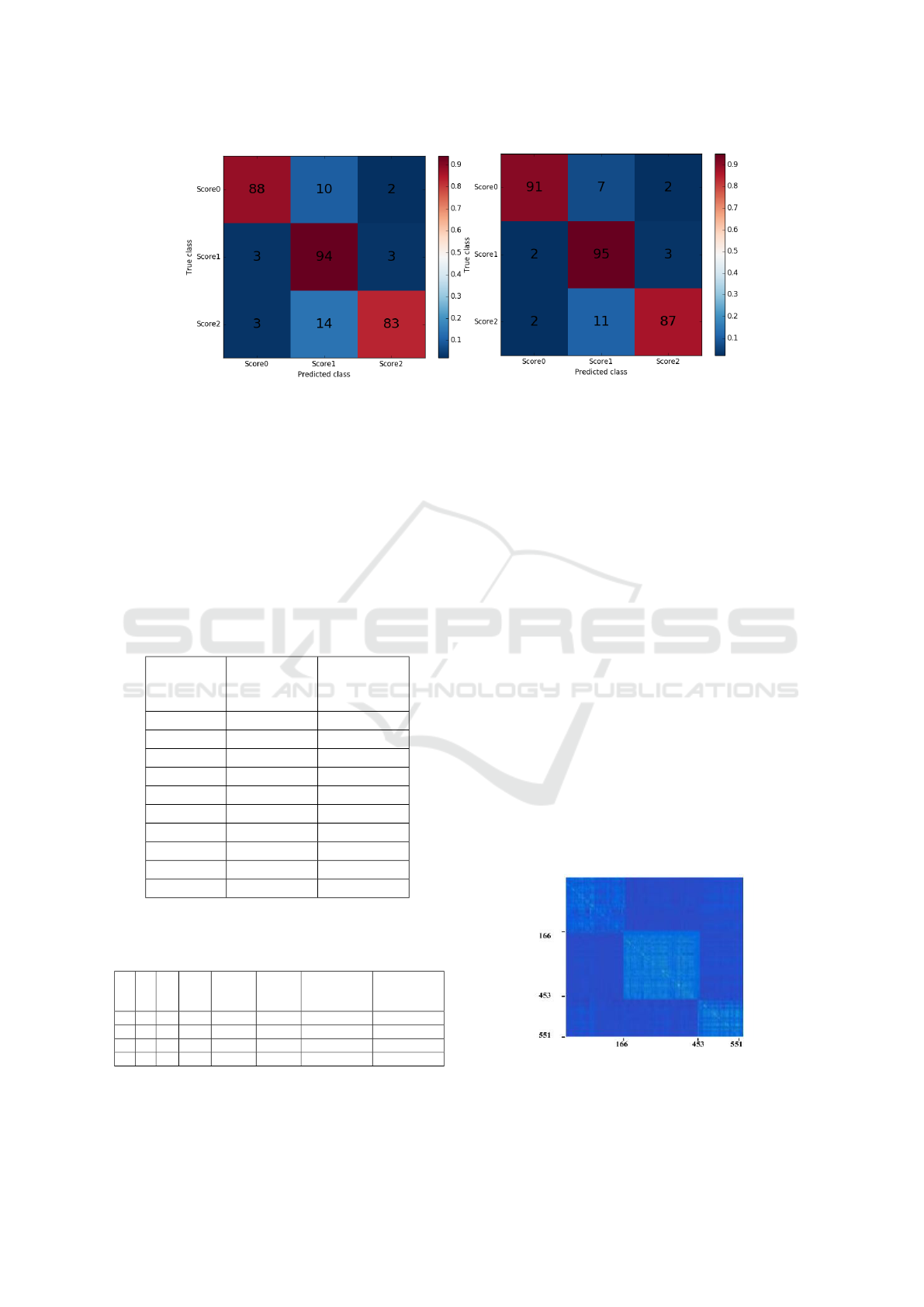
(a) HOF (b) MBH
Figure 6: Confusion matrix of HOF and MBH feature vector using GMM-IMK dynamic kernel with SVM for 256 components
for 3-class grading scores (best viewed in color).
expressions from the previous works are compared,
this is due to the previous works only focus on the ex-
pressions which have notable (eminent/distinguished)
facial movements like wrinkle forehead (EP1), clo-
sure of eye tightly (EP3), wrinkle nose (EP5), and grin
(EP7). This is evaluated to facilitate the comparison
with the previous work.
Table 8: Expression wise classification performance (%) of
the proposed approach for the best model (MBH features
using MIK kernel for 256 components.
Expression
Denotations
Proposed
5-score
grading score
Proposed
3-score
grading score
EP0 75.45 81.68
EP1 95.23 94.87
EP2 86.44 93.04
EP3 91.94 97.43
EP4 94.13 92.3
EP5 95.97 95.6
EP6 91.57 91.94
EP7 93.77 95.23
EP8 89.01 87.54
EP9 93.04 95.23
Table 9: Comparison of the classification performance (%)
for the few prominent facial paralysis expressions with the
existing works.
PI LBPGabor
Tracking
2D
Tracking
3D
Proposed
5-class
grading scores
Proposed
3-class
grading scores
EP150.7 58.3 62.4 69.4 70.9 95.23 94.87
EP348.2 48.9 53.1 62.1 63.3 91.94 97.43
EP548.1 41.8 50.5 57.3 58.2 95.97 95.6
EP739.2 40.1 54.5 70.6 73.5 93.77 95.23
4.4 Efficacy of the Proposed Approach
Figure 7 shows the visualization of the kernel matrix
of the best performing MBH features with a mean in-
terval kernel (MIK) for 256 components and 3-class
grading score. The lighter shade of the diagonal ele-
ments show the higher values, which represents the
correctly classified elements while the off-diagonal
elements in darker shade represent the lower values.
Also, it can be inferred that using MIK as a distance
metric there is better separability among the different
levels of the facial paralysis.
Further, it can be observed from Table 8, expres-
sions like at rest (EP0) and closure of eye lightly
(EP2), where there are few or no facial movements
results in low performance of the proposed approach.
Also, from figures 8 (a) and 8 (b), it can be observed
that expressions having common facial movements
like blowing out cheeks (EP6) and whistling (EP8)
are confused with each other. And expression hav-
ing distinguished (uncommon) facial movements like
wrinkle forehead (EP1) and wrinkle nose (EP5) are
less confused with each other.
Figure 7: Mean interval kernel representation for motion
boundary histogram (MBH) features and uGMM 256 com-
ponents and 3-class grading score (best viewed in color).
VISAPP 2020 - 15th International Conference on Computer Vision Theory and Applications
182

(a) (b)
Figure 8: t-sne plot for the expressions of facial paralysis
using MBH and GMM-MIK dynamic kernel based SVM
for 256 components for 3-class grading score (best viewed
in color). In (a) t-sne plot for expression blowing out cheeks
(EP6) and whistling (EP8) and in (b) for expression wrinkle
forehead (EP1) and wrinkle nose (EP5).
5 CONCLUSION
In this paper, we introduce a novel representation
of the facial features for variable length pattern us-
ing dynamic kernel-based classification, which pro-
vide the quantitative assessment to the patients suffer-
ing from facial paralysis. Dynamic kernels are used
for representing the varying length videos efficiently
by capturing both local facial dynamics and preserv-
ing the global context. A universal Gaussian mixture
model (GMM) is trained on spatio-temporal features
to compute the posteriors, first-order, and second-
order statistics for computing dynamic kernel-based
representations. We have shown that the efficacy of
the proposed approach using different dynamic ker-
nels on the collected video dataset of facially par-
alyzed patients. Also, we have shown the compu-
tation complexity and classification performance of
each dynamic kernels, where the matching based in-
termediate matching kernel (IMK) is computationally
efficient as compared to other dynamic kernels. How-
ever, probability-based mean interval kernel (MIK) is
more discriminative but computationally complex. In
the future, the classification performance has to be im-
proved further by improving the modeling of expres-
sions for better quantitative assessment of the facial
paralysis. Also, various quantitative assessment using
Perveen et al. (2012); Perveen et al. (2018); Perveen
et al. (2016) are need to be explore and compare for
better classification performance.
REFERENCES
Banks, C. A., Bhama, P. K., Park, J., Hadlock, C. R., and
Hadlock, T. A. (2015). Clinician-Graded Electronic
Facial Paralysis Assessment: The eFACE. Plast. Re-
constr. Surg., 136(2):223e–230e.
Cortes, C. and Vapnik, V. (1995). Support-vector networks.
Machine Learning, 20(3):273–297.
Dileep, A. D. and Sekhar, C. C. (2014). Gmm-based inter-
mediate matching kernel for classification of varying
length patterns of long duration speech using support
vector machines. IEEE Transactions on Neural Net-
works and Learning Systems, 25(8):1421–1432.
Guo, Z., Shen, M., Duan, L., Zhou, Y., Xiang, J., Ding, H.,
Chen, S., Deussen, O., and Dan, G. (2017). Deep as-
sessment process: Objective assessment process for
unilateral peripheral facial paralysis via deep con-
volutional neural network. In 2017 IEEE 14th In-
ternational Symposium on Biomedical Imaging (ISBI
2017), pages 135–138.
Hato, N., Fujiwara, T., Gyo, K., and Yanagihara, N. (2014).
Yanagihara facial nerve grading system as a prognos-
tic tool in Bell’s palsy. Otol. Neurotol., 35(9):1669–
1672.
He, S., Soraghan, J. J., O’Reilly, B. F., and Xing, D. (2009).
Quantitative analysis of facial paralysis using local bi-
nary patterns in biomedical videos. IEEE Transac-
tions on Biomedical Engineering, 56(7):1864–1870.
House, J. W. and Brackmann, D. E. (1985). Facial nerve
grading system. Otolaryngology-Head and Neck
Surgery, 93(2):146–147. PMID: 3921901.
Liu, X., Dong, S., An, M., Bai, L., and Luan, J. (2015).
Quantitative assessment of facial paralysis using in-
frared thermal imaging. In 2015 8th International
Conference on Biomedical Engineering and Informat-
ics (BMEI), pages 106–110.
NGO, T. H., CHEN, Y.-W., MATSUSHIRO, N., and SEO,
M. (2016). Quantitative assessment of facial paralysis
based on spatiotemporal features. IEICE Transactions
on Information and Systems, E99.D(1):187–196.
Ngo, T. H., Chen, Y. W., Seo, M., Matsushiro, N., and
Xiong, W. (2016). Quantitative analysis of facial
paralysis based on three-dimensional features. In 2016
IEEE International Conference on Image Processing
(ICIP), pages 1319–1323.
Ngo, T. H., Seo, M., Chen, Y.-W., and Matsushiro, N.
(2014). Quantitative assessment of facial paralysis us-
ing local binary patterns and gabor filters. In Proceed-
ings of the Fifth Symposium on Information and Com-
munication Technology, SoICT ’14, pages 155–161,
New York, NY, USA. ACM.
Perveen, N., Gupta, S., and Verma, K. (2012). Facial ex-
pression recognition using facial characteristic points
and gini index. In 2012 Students Conference on Engi-
neering and Systems, pages 1–6.
Perveen, N., Roy, D., and Mohan, C. K. (2018). Sponta-
neous expression recognition using universal attribute
model. IEEE Transactions on Image Processing,
27(11):5575–5584.
Perveen, N., Singh, D., and Mohan, C. K. (2016). Sponta-
neous facial expression recognition: A part based ap-
proach. In 2016 15th IEEE International Conference
on Machine Learning and Applications (ICMLA),
pages 819–824.
Satoh, Y., Kanzaki, J., and Yoshihara, S. (2000). A com-
parison and conversion table of ’the house-brackmann
Quantitative Analysis of Facial Paralysis using GMM and Dynamic Kernels
183

facial nerve grading system’ and ’the yanagihara grad-
ing system’. Auris Nasus Larynx, 27(3):207 – 212.
Tran, D., Bourdev, L. D., Fergus, R., Torresani, L., and
Paluri, M. (2014). C3D: generic features for video
analysis. CoRR, abs/1412.0767.
Wachtman, G., Liu, Y., Zhao, T., Cohn, J., Schmidt, K.,
Henkelmann, T., VanSwearingen, J., and Manders, E.
(2002). Measurement of asymmetry in persons with
facial paralysis. In Combined Annual Conference of
the Robert H. Ivy and Ohio Valley societies of Plastic
and Reconstructive Surgeons.
Wang, H., Oneata, D., Verbeek, J., and Schmid, C. (2015).
A robust and efficient video representation for action
recognition. International Journal of Computer Vi-
sion, 119(3):219–238.
VISAPP 2020 - 15th International Conference on Computer Vision Theory and Applications
184
