Modelling Brain Lesion Volume in Patches with CNN-based Poisson

Regression

Kevin Raina

Department of Mathematics and Statistics, University of Ottawa, Ontario, Canada

Keywords:

Stroke, Brain Lesions, MRI, Poisson Regression (PR), Convolutional Neural Network.

Abstract:

Monitoring the progression of lesions is important for clinical response. Summary statistics such as lesion

volume are objective and easy to interpret, which can help clinicians assess lesion growth or decay. CNNs are

commonly used in medical image segmentation for their ability to produce useful features within large con-

texts and their associated efﬁcient iterative patch-based training. Many CNN architectures require hundreds

of thousands parameters to yield a good segmentation. In this work, an efﬁcient, computationally inexpensive

CNN is implemented to estimate the number of lesion voxels in a predeﬁned patch size from magnetic reso-

nance (MR) images. The output of the CNN is interpreted as the conditional Poisson parameter over the patch,

allowing standard mini-batch gradient descent to be employed. The ISLES2015 (SISS) data is used to train

and evaluate the model, which by estimating lesion volume from raw features, accurately identiﬁed the lesion

image with the larger lesion volume for 86% of paired sample patches. An argument for the development and

use of estimating lesion volumes to also aid in model selection for segmentation is made.

1 INTRODUCTION

Many segmentation challenges have been undertaken

recently, showing the need for automated models in

clinical settings (Maier et al., 2017; Winzeck et al.,

2018; Bakas et al., 2018). Along with strong predic-

tive power, these challenges stress the importance of

fast inference, as lesions can quickly spread. For in-

stance, ischemic stroke lesions cause increasing tis-

sue death within hours of onset, requiring reperfu-

sion therapies around this time. The stroke progresses

through acute, sub-acute and chronic stages within

days. Gliomas, the most common type of malignant

brain tumour, grows at a rate of increasing severity

depending on the grade. As the tumour gets larger,

symptoms often worsen, reinforcing the need to mon-

itor lesion growth.

A simple, yet powerful, summary statistic is the

lesion volume, or when the brain is represented as

labelled voxels, the lesion label count. In a clini-

cal study, (Alexander et al., 2010) showed that le-

sion volume is a signiﬁcant covariate for understand-

ing ischemic stroke deﬁcits after the initial onset. In

application, lesion volume has generally been a de-

pendable factor in the prognosis of ischemic stroke

https://orcid.org/0000-0002-6240-9675

(Merino et al., 2007; Rivers et al., 2006) and multi-

ple sclerosis (Zivadinov et al., 2012; Bagnato et al.,

2011). The objectivity of counts enables straightfor-

ward inference: a higher lesion label count means the

lesion has grown.

In comparison to segmenting entire 3D medical

images, directly estimating the number of lesion vox-

els in the brain from raw features should be expected

to require less computational resources since it is

no longer necessary to provide detailed information

about the lesion’s appearance. Nonetheless, in a study

by (Erskine et al., 2005) comparing the effects on vol-

ume estimation by using different magnetic resonance

imaging scanners, lesion volume was estimated from

a computer-assisted segmentation tool. Other meth-

ods for estimating lesion volume favored a geometric

approach, wherein the lesion’s surface area per slice is

calculated and the estimate is derived by summing ac-

cross slices (Park et al., 2013; Filippi et al., 1995). In

contrast, the output of our proposed statistical direct

lesion counting model is a single non-negative integer

that doesn’t require sophisticated viewing software or

signiﬁcant memory usage.

CNNs have shown promising results in lesion seg-

mentation, as in the works of (Kamnitsas et al., 2017),

(Havaei et al., 2017) and (Ronneberger et al., 2015),

due to their ability to produce useful features from

172

Raina, K.

Modelling Brain Lesion Volume in Patches with CNN-based Poisson Regression.

DOI: 10.5220/0009102701720176

In Proceedings of the 13th International Joint Conference on Biomedical Engineering Systems and Technologies (BIOSTEC 2020) - Volume 2: BIOIMAGING, pages 172-176

ISBN: 978-989-758-398-8; ISSN: 2184-4305

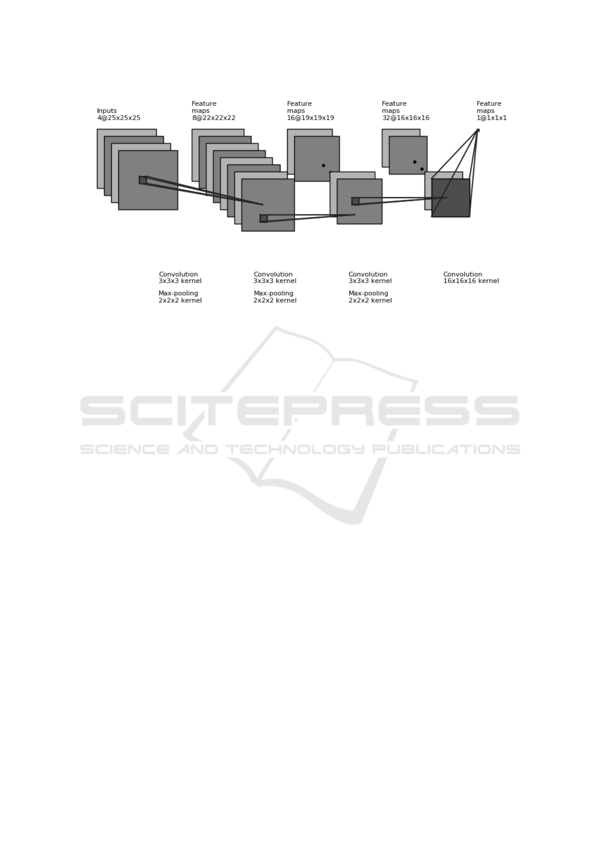
Figure 1: 3D architecture employed for counting lesions. The input tensor is obtained by stacking patches from the patient’s

brain MRI over 4 different modalities. After applying convolution and pooling operations, the ﬁnal output is a real number.

large visual spatial contexts combined with efﬁcient

iterative patch-based training and dense inference.

The output of the CNN is often interpeted as the pa-

rameter of a conditional distribution. For instance, in

(Kamnitsas et al., 2017; Havaei et al., 2017), the out-

put at each voxel is the parameter of a Bernoulli con-

ditional distribution. The Poisson distribution is gen-

erally well known for modelling counts over time and

space, and particularly has been applied to modelling

the count of multiple sclerosis lesions over time (Alt-

man and Petkau, 2005; Albert et al., 1994). For this

reason, we propose the lesion label counts, or equiv-

alently lesion volume, in a predeﬁned patch size is

assumed to follow a Poisson distribution conditional

on the patch features. The CNNs of (Kamnitsas et al.,

2017) and (Havaei et al., 2017) use hundreds of thou-

sands of parameters for segmentation. Using CNNs,

coupled with good distributional assumptions, should

allow for smaller architectures and faster convergence

on the counting task.

One prior related work by (Dubost et al., 2017)

used a 3D CNN, similar to U-Net (Ronneberger et al.,

2015) to predict global lesion label count, but pro-

duces a segmentation when testing by using a remov-

able global pooling layer. A drawback of estimating

global lesion label counts is the need for more pa-

tient brain images, since an entire brain serves as a

single sample. In their study, training was performed

on 1,289 3D PD-weighted MRI scans, whereas some

challenges provide limited training instances (Maier

et al., 2017). Another challenge with global lesion

counts is being able to efﬁciently produce scalar out-

puts from larger 3D information, which would require

additional preprocessing and transformations. Esti-

mation of counts in patches can help in these situa-

tions.

This paper is organized as follows: Section 2 de-

scribes the methods, Section 3 presents the results,

and a discussion follows in Section 4.

2 METHODS

2.1 Architecture

The proposed network is shown in Figure 1. As in-

put it stacks 25 × 25 × 25 patches from each MR se-

quence, runs 3 layers of convolution and max pooling

which have sizes 3 × 3 × 3 and 2 × 2 × 2 respectively,

followed by a ﬁnal convolution of size 16 ×16 ×16 to

output one real number. In addition to the convolution

and max pooling operations, Leaky ReLU nonlinear-

ity was used. It is important to note the number of

output activations at each layer are considerably small

to reduce the total number of parameters. The patch is

not only a parameter of the training features, but is in-

tertwined with the task as well, since it delineates the

region over which the lesion label count is estimated.

Training: A block diagram of the methodology is

shown in Figure 2. In accordance with the notation

of Figure 2, the architecture associates one real num-

ber N to each input tensor. Then, the model can be

formulated as: c|X ∼ Pois(e

N(X ,Θ)

), where c is the

lesion label count over the patch, X are the input fea-

Modelling Brain Lesion Volume in Patches with CNN-based Poisson Regression

173

Figure 2: Block diagram representation of the CNN-based Poisson Regression model. The predicted count is obtained by

ﬂooring the estimated conditional Poisson parameter (λ).

tures used in the architecture, and Θ are the param-

eters of the architecture. In order to train the pa-

rameters from observed counts c

(assumed to Pois-

son distributed with rate λ

), mini-batch gradient de-

scent with a batch size b is used to minimize the

average negative log-likelihood, −

∑

i=1

log(

−λ

plus additional L1 and L2 regularization terms to pre-

vent overﬁtting. The samples used in the mini-batch

were taken so as to ensure the lesion count was non-

zero by insisting the central voxel be lesion. Since

training only samples non-zero counts, it will not be

efﬁcient at predicting counts for completely randomly

sampled patches, for which zero counts are more fre-

quent. A possible workaround for this task is using

a zero-inﬂated Poisson model (ZIP) (Lambert, 1992),

which is suggested for a future study.

2.2 Implementation Details

The open-source software Tensorﬂow was used to

implement the model (Abadi et al., 2016). Non-

zero counts were sampled in mini-batches of size 10.

Weights were initialized under a Gaussian with mean

0 and standard deviation of 0.001, while biases are

initialized to 0. Moreover, the Adam Optimizer was

used with initial learning rate of 10

−4

, and training

was stopped when the average cost over 1, 000 itera-

tions increased. This always happened within 15,000

iterations. In comparison, the segmentation CNN of

(Kamnitsas et al., 2017) has default training conﬁgu-

rations set to 70,000 iterations, demonstrating a quick

ability to learn for direct counting models. L1 regu-

larization and L2 regularization were used and set to

−8

and 10

−6

respectively. In addition to regulariza-

tion, dropout on all hidden layers was employed at a

rate ot 0.5. At prediction time, the mean Poisson rate

was ﬂoored to provide an integer estimate. Table 1

summarizes the implementation details.

3 EXPERIMENTS AND RESULTS

3.1 Dataset

The architecture and model were trained and evalu-

ated on the ISLES2015 (SISS) training data, which

Table 1: Numerical summary of implementation details.

Implementation Detail Value

Batch size (b) 10

Kernel initialization mean(std.) 0(0.001)

Learning rate 10

−4

L1, L2 coefﬁcients 10

−8

,10

−6

Dropout 0.5

consists of 28 patients with sub-acute ischemic stroke.

All data come from the same clinical center, which

provided 4 MR sequences for each patient: FLAIR,

DWI, T1 and T1-contrast. Images are of size 230 ×

230 × 153/154, are processed to not contain the skull

and have isotropic 1mm

voxel resolution. Sub-acute

ischemic stroke lesions have large variation in size.

For instance, in the dataset, the smallest lesion con-

sists of 106 voxels, and the largest consists of 233,547

voxels. From the 28 brains, 20 were randomly se-

lected to form the training set, and the remaining 8

formed the validation set. This selection was carried

out once, and the same split was used across all ex-

periments. It should be acknowledged that the choice

of the training and validation split will have an effect

on performance due to the aformentioned variability

in lesion count.

3.2 Model Performance

To evaluate the performance of the architecture, sev-

eral metrics are calculated on 10,000 patches sampled

to have a non-zero lesion label count from the valida-

tion set. Sampling was done by ﬁrst selecting the vali-

dation brain and then selecting a patch from the brain.

Estimated counts that surpassed the possible count in

the predeﬁned patch size were adjusted to predict the

maximum possible count. In the experiment applied

to the ISLES2015 (SISS) data, the mean absolute er-

ror (MAE) rounded up to the nearest integer was com-

puted to be 1,458. In addition, over the same samples

the average estimated count to true count ratio was

computed to be 1.15. Finally, the mean relative error

(MRE) was 0.42 for the ischemic stroke lesions. True

patch lesion label counts vary from a few hundred to

15,000, indicating a promising initial result. Figure 3

plots the estimated and true counts for 200 samples.

BIOIMAGING 2020 - 7th International Conference on Bioimaging

174

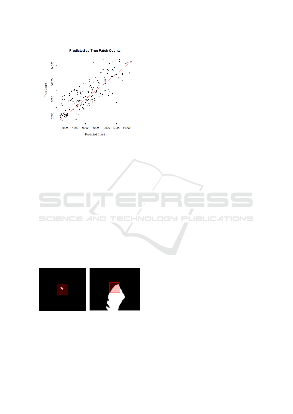
Figure 3: Plot of true count and estimated count for 200

lesion patch samples. Coefﬁcient of multiple correlation

(Pearson’s correlation coefﬁcient between predicted and ac-

tual values) of R = 0.81.

3.3 Predicting Count Order

The second experiment was to order pairs of patches

by lesion label count, which can be applied in a clin-

ical setting to compare lesion images over time and

assess growth or decay. Given any two image patches

containing lesions, the goal is to evaluate the model’s

ability to identify the image with the larger (equiva-

lently smaller) lesion volume using the proposed esti-

mation. In the experiment, 10,000 pairs of non-zero

count patches are sampled from the validation fold. A

sample is counted as correct if the predicted counts

preserve the same order as the true counts. Running

the experiment on the ISLES2015 (SISS) data gives a

correct order prediction for 86 % of samples, demon-

strating good ordering capabilities. Figure 4 shows an

accurately predicted sample.

Figure 4: Example of predicting count order, where the red

square outline represents the middle slice of the 25

patch.

The true counts from left to right are: 356 and 5297. The

predicted counts from left to right are: 501 and 5640. In

this case, the model accurately identiﬁes the left image as

having the smaller lesion volume.

4 FUTURE WORK

4.1 Extension to Arbitrary Patches

The analysis and modelling undertaken in the previ-

ous sections were done on patches that contain lesion

voxels. That is, the patches were sampled to contain

lesion voxels. Although it was shown that this has the

potential for modelling lesion growth or decay by ﬁrst

estimating lesion volume, relaxing this restriction al-

lows for the prediction of counts in arbitrary patches,

which are more frequently zero counts. Due to the un-

balanced nature of the data, one proposition for a fu-

ture study is to combine a zero-inﬂated Poisson model

which is known to account for excess zero counts in

data, with CNNs.

4.2 Location Detection

Being able to predict counts in arbitrary patches can

form the basis for lesion location detection. A pos-

sible algorithm could be to randomly sample patches

from one brain, predict their counts, and record the

central voxel position for the patch with the maxi-

mum predicted count. The voxel position returned

by the algorithm should identify an area of signiﬁ-

cant lesion presence in the brain, assuming the model

is well-tuned. Though simple, the algorithm is theo-

retically stable when applied on a single lesion, since

applying true counts in place of predictions will al-

ways return the location of a lesion provided a lesion

is present.

Rather than recording just the maximum predicted

count from the given sample, another option would be

to order the predicted counts for samples drawn from

one brain. From a pre-deﬁned quantile, larger counts

a long with their central voxel positions will delineate

the lesion.

4.3 Model Selection for Segmentation

The size of a lesion is one of the factors that can

allow some conﬁgurations of a segmentation algo-

rithm to perform better than others (Kamnitsas et al.,

2017). Smaller lesions, often found in sub-acute is-

chemic stroke, are usually tougher to segment and

produce lower dice coefﬁcients (Havaei et al., 2017)

than larger lesions due to a relatively higher num-

ber of false positives compared to true positives. For

CNNs, conﬁgurations mainly pertain to the architec-

ture employed. Given that some architectures may

segment smaller lesions better, one option is to regress

the architecture employed for a brain, on an estimate

of the global lesion label count in the brain.

Modelling Brain Lesion Volume in Patches with CNN-based Poisson Regression

175

5 DISCUSSION

Direct counting models might be useful in clinical

settings. Some potential examples are but not lim-

ited to: monitoring and locating lesions. They can

also aid segmentation by selecting conﬁgurations of

segmentation algorithms based on global lesion size,

from raw data, and reducing the required segmenta-

tion area through lesion detection. Further develop-

ments need to be made to predict patch counts, includ-

ing: improving accuracy in the predictions of non-

zero counts, accounting for highly imbalanced zero

counts, developing sampling-based algorithms for le-

sion location detection, and providing aggregate patch

measures to predict global lesion count. This will in-

crease the effectiveness and broaden the applications

of direct counting models.

REFERENCES

Abadi, M., Barham, P., Chen, J., Chen, Z., Davis, A., Dean,

J., Devin, M., Ghemawat, S., Irving, G., Isard, M.,

et al. (2016). Tensorﬂow: a system for large-scale

machine learning. In OSDI, volume 16, pages 265–

283.

Albert, P. S., McFarland, H. F., Smith, M. E., and Frank,

J. A. (1994). Time series for modelling counts from a

relapsing-remitting disease: application to modelling

disease activity in multiple sclerosis. Statistics in

Medicine, 13(5-7):453–466.

Alexander, L. D., Black, S. E., Gao, F., Szilagyi, G.,

Danells, C. J., and McIlroy, W. E. (2010). Correlat-

ing lesion size and location to deﬁcits after ischemic

stroke: the inﬂuence of accounting for altered peri-

necrotic tissue and incidental silent infarcts. Behav-

ioral and brain functions, 6(1):6.

Altman, R. M. and Petkau, A. J. (2005). Application of hid-

den markov models to multiple sclerosis lesion count

data. Statistics in Medicine, 24(15):2335–2344.

Bagnato, F., Ikonomidou, V. N., van Gelderen, P., Auh,

S., Hanafy, J., Cantor, F. K., Ohayon, J., Richert,

N., and Duyn, J. (2011). Lesions by tissue speciﬁc

imaging characterize multiple sclerosis patients with

more advanced disease. Multiple Sclerosis Journal,

17(12):1424–1431.

Bakas, S., Reyes, M., Jakab, A., Bauer, S., Rempﬂer, M.,

Crimi, A., Shinohara, R. T., Berger, C., Ha, S. M.,

Rozycki, M., et al. (2018). Identifying the best ma-

chine learning algorithms for brain tumor segmen-

tation, progression assessment, and overall survival

prediction in the brats challenge. arXiv preprint

arXiv:1811.02629.

Dubost, F., Bortsova, G., Adams, H., Ikram, A., Niessen,

W. J., Vernooij, M., and De Bruijne, M. (2017). Gp-

unet: Lesion detection from weak labels with a 3d

regression network. In International Conference on

Medical Image Computing and Computer-Assisted In-

tervention, pages 214–221. Springer.

Erskine, M., Cook, L., Riddle, K., Mitchell, J. R., and Kar-

lik, S. J. (2005). Resolution-dependent estimates of

multiple sclerosis lesion loads. Canadian journal of

neurological sciences, 32(2):205–212.

Filippi, M., Horsﬁeld, M., Campi, A., Mammi, S., Pereira,

C., and Comi, G. (1995). Resolution-dependent esti-

mates of lesion volumes in magnetic resonance imag-

ing studies of the brain in multiple sclerosis. Annals

of Neurology: Ofﬁcial Journal of the American Neuro-

logical Association and the Child Neurology Society,

38(5):749–754.

Havaei, M., Davy, A., Warde-Farley, D., Biard, A.,

Courville, A., Bengio, Y., Pal, C., Jodoin, P.-M., and

Larochelle, H. (2017). Brain tumor segmentation

with deep neural networks. Medical image analysis,

35:18–31.

Kamnitsas, K., Ledig, C., Newcombe, V. F., Simpson,

J. P., Kane, A. D., Menon, D. K., Rueckert, D., and

Glocker, B. (2017). Efﬁcient multi-scale 3D CNN

with fully connected CRF for accurate brain lesion

segmentation. Medical image analysis, 36:61–78.

Lambert, D. (1992). Zero-inﬂated poisson regression, with

an application to defects in manufacturing. Techno-

metrics, 34(1):1–14.

Maier, O., Menze, B. H., von der Gablentz, J., H

ani, L.,

Heinrich, M. P., Liebrand, M., Winzeck, S., Basit, A.,

Bentley, P., Chen, L., et al. (2017). ISLES 2015 - a

public evaluation benchmark for ischemic stroke le-

sion segmentation from multispectral MRI. Medical

image analysis, 35:250–269.

Merino, J. G., Latour, L. L., Todd, J. W., Luby, M.,

Schellinger, P. D., Kang, D.-W., and Warach, S.

(2007). Lesion volume change after treatment with

tissue plasminogen activator can discriminate clinical

responders from nonresponders. Stroke, 38(11):2919–

2923.

Park, H.-J., Machado, A. G., Cooperrider, J., Truong-

Furmaga, H., Johnson, M., Krishna, V., Chen, Z., and

Gale, J. T. (2013). Semi-automated method for esti-

mating lesion volumes. Journal of neuroscience meth-

ods, 213(1):76–83.

Rivers, C., Wardlaw, J., Armitage, P., Bastin, M., Carpen-

ter, T., Cvoro, V., Hand, P., and Dennis, M. (2006).

Do acute diffusion-and perfusion-weighted mri le-

sions identify ﬁnal infarct volume in ischemic stroke?

Stroke, 37(1):98–104.

Ronneberger, O., Fischer, P., and Brox, T. (2015). U-net:

Convolutional networks for biomedical image seg-

mentation. In International Conference on Medical

image computing and computer-assisted intervention,

pages 234–241. Springer.

Winzeck, S., Hakim, A., McKinley, R., Pinto, J. A., Alves,

V., Silva, C., Pisov, M., Krivov, E., Belyaev, M.,

Monteiro, M., et al. (2018). ISLES 2016 and 2017-

benchmarking ischemic stroke lesion outcome predic-

tion based on multispectral MRI. Frontiers in neurol-

ogy, 9.

Zivadinov, R., Heininen-Brown, M., Schirda, C. V., Poloni,

G. U., Bergsland, N., Magnano, C. R., Durfee, J.,

Kennedy, C., Carl, E., Hagemeier, J., et al. (2012).

Abnormal subcortical deep-gray matter susceptibility-

weighted imaging ﬁltered phase measurements in pa-

tients with multiple sclerosis: a case-control study.

Neuroimage, 59(1):331–339.

BIOIMAGING 2020 - 7th International Conference on Bioimaging

176