Monocular 3D Object Detection via Geometric Reasoning on Keypoints

Ivan Barabanau

, Alexey Artemov

, Evgeny Burnaev

and Vyacheslav Murashkin

Skolkovo Institute of Science and Technology, Moscow, Russia

Yandex.Taxi, Moscow, Russia

Keywords:

Deep Learning, Monocular Vision, 3D Object Detection.

Abstract:

Monocular 3D object detection is well-known to be a challenging vision task due to the loss of depth in-

formation; attempts to recover depth using separate image-only approaches lead to unstable and noisy depth

estimates, harming 3D detections. In this paper, we propose a novel keypoint-based approach for 3D object

detection and localization from a single RGB image. We build our multi-branch model around 2D keypoint

detection in images and complement it with a conceptually simple geometric reasoning method. Our network

performs in an end-to-end manner, simultaneously and interdependently estimating 2D characteristics, such as

2D bounding boxes, keypoints, and orientation, along with full 3D pose in the scene. We fuse the outputs of

distinct branches, applying a reprojection consistency loss during training. The experimental evaluation on the

challenging KITTI dataset benchmark demonstrates that our network achieves state-of-the-art results among

other monocular 3D detectors.

1 INTRODUCTION

The success of autonomous robotics systems, such

as self-driving cars, largely relies on their ability to

operate in complex dynamic environments; as an es-

sential requirement, autonomous systems must reli-

ably identify and localize non-stationary and interact-

ing objects, e.g. vehicles, obstacles, or humans. In its

simplest formulation, localization is understood as an

ability to detect and frame objects of interest in 3D

bounding boxes, providing their 3D locations in the

surrounding space. Crucial to the decision-making

process is the accuracy of depth estimates of the 3D

detections.

Depth estimation could be approached from both

hardware and algorithmic perspectives. On the sen-

sors end, laser scanners such as LiDAR devices have

been extensively used to acquire depth measurements

sufﬁcient for 3D detection in many cases (Yang et al.,

2018; Chen et al., 2017; Lang et al., 2019; Zhou and

Tuzel, 2018; Ku et al., 2018; Yan et al., 2018). How-

ever, point clouds produced by these expensive sen-

sors are sparse, noisy and massively increase mem-

ory footprints with millions of 3D points acquired per

second. In contrast, image-based 3D detection meth-

ods offer savings on CPU and memory consumption,

use cheap onboard cameras, and work with a wealth

of established detection architectures (e.g., (Liu et al.,

2016; Redmon et al., 2016; Ren et al., 2015; Lin et al.,

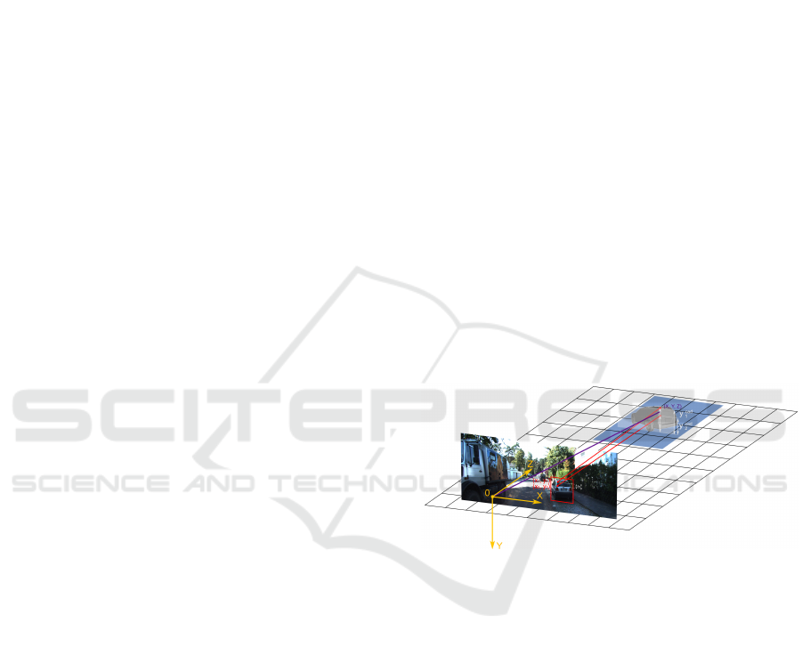
Figure 1: Geometric reasoning about instance depth (best

viewed in zoom). We use camera intrinsic parameters, pre-

dict 2D keypoints and infer dimensions to “lift” the key-

points to 3D space.

2017a; He et al., 2017; Lin et al., 2017b; Liu et al.,

2018; Simonelli et al., 2019)), yet they require sophis-

ticated algorithms for depth estimation, as raw depth

cannot be accessed anymore.

Recent research on monocular 3D object detection

relies on separate dense depth estimation models (Qin

et al., 2019; Xu and Chen, 2018), but depth recovery

from monocular images is naturally ill-posed, leading

to unstable and noisy estimates. In addidion, in many

practical instances, e.g., with sufﬁcient target resolu-

tion or visibility, dense depth estimation might be re-

dundant in context of 3D detection. Instead, one may

focus on obtaining sparse but salient features, such

as 2D keypoints, that are well-known visual cues of-

ten serving as geometric constrains in various vision

tasks such as human pose estimation (Ramakrishna

652

Barabanau, I., Artemov, A., Burnaev, E. and Murashkin, V.

Monocular 3D Object Detection via Geometric Reasoning on Keypoints.

DOI: 10.5220/0009102506520659

In Proceedings of the 15th International Joint Conference on Computer Vision, Imaging and Computer Graphics Theory and Applications (VISIGRAPP 2020) - Volume 5: VISAPP, pages

652-659

ISBN: 978-989-758-402-2; ISSN: 2184-4321

et al., 2012; Martinez et al., 2017; Mehta et al., 2017a;

Mehta et al., 2017b) and more general object interpre-

tation (Hejrati and Ramanan, 2012; Wu et al., 2016).

Motivated by this observation, in this paper we

propose a novel keypoint-based approach for 3D ob-

ject detection and localization from a single RGB im-

age. We build our model around 2D keypoint detec-

tion in images and complement it with a conceptually

simple geometric reasoning framework, establishing

correspondences between the detected 2D keypoints

and their 3D counterparts deﬁned on surfaces of 3D

CAD models. The framework operates under the gen-

eral assumptions, assuming the camera intrinsic pa-

rameters are given, and retrieves depth of closest key-

point instance to ”lift” 2D keypoints to 3D space; the

remaining 3D keypoints and the ﬁnal 3D detection are

assembled in a similar way. To enhance robustness

of our 2D keypoint detection, we use a multi-task re-

projection consistency loss; our model is ultimately

end-to-end trainable. Additionally, our approach does

not require images manually labelled with keypoints,

but instead uses annotations automatically obtained

from back-projecting data-aligned CAD models from

3D space to the image plane; we only mark 14 3D

keypoints per each of 5 3D CAD models, totalling

70 manually labelled 3D keypoints, which makes our

approach particularly labour-efﬁcient in terms of an-

notation costs.

In summary, our contributions are as follows:

• We propose a novel deep learning-based frame-

work for monocular 3D object detection, combin-

ing well-established region-based detectors and a

geometric reasoning step over inferred keypoints.

• We create keypoint annotations for images

in the KITTI 3D object detection benchmark

dataset (Geiger et al., 2012; Geiger et al., 2013),

using a collection of 3D CAD models, annotated

with 3D keypoints. We note that the dataset is

obtained without any human labour. We describe

how to train our framework in an end-to-end fash-

ion using the newly created annotations.

2 RELATED WORK

The most relevant to our work is research on monoc-

ular 3D object detection, that is well-known to be

a challenging vision task. Deep3DBox (Mousavian

et al., 2017) relies on a set of geometric constraints

between 2D and predicted 3D bounding boxes and

reduces 3D object localization problem to a linear

system of equations, ﬁtting 3D box projections into

2D detections. Their approach relies on a separate

linear solver; in contrast, our model is end-to-end

trainable and does not require external optimization.

Mono3D (Chen et al., 2016) extensively samples 14K

3D bounding box proposals per image and evaluates

each, exploiting semantic and image-based features.

In contrast, our approach does not rely on an exhaus-

tive sampling in 3D space, bypassing a signiﬁcant

computational overhead. OFT-Net (Roddick et al.,

2018) introduces an orthographic feature transform

which maps RGB image features into a birds-eye-

view representation through a 3D scene grid, solv-

ing the perspective projection problem. However,

back-projecting image features onto 3D grid results

in a coarse feature assignment. Our approach de-

tects 2D keypoints with sufﬁcient precision, avoid-

ing any additional discretization. MonoGRNet (Qin

et al., 2019) directly deals with depth estimation from

a single image, training an additional sub-network to

predict the z-coordinate of each 3D bounding box.

(Xu and Chen, 2018) exploit a similar approach, esti-

mating disparity using a stand-alone pre-trained Mon-

oDepth network (Godard et al., 2017). Both these

methods rely on the non-trainable depth estimation

networks, which introduce a computational overhead;

in contrast to (Xu and Chen, 2018) and (Godard

et al., 2017), our approach jointly estimates object 2D

bounding-box and 3D pose in a fully trainable man-

ner, not requiring a dense depth prediction and is sim-

ilar in this respect to (Qin et al., 2019).

Perhaps, the most similar approach to ours

is (Chabot et al., 2017), which utilizes 3D CAD mod-

els, along with predicting 2D keypoints. However,

their network only models 2D geometric properties

and aims at matching the predictions to one of the

CAD shapes, while 3D pose estimation is postponed

for the inference step. They additionally exploit ex-

tensive annotations of keypoints in their 3D models.

In contrast, we only annotate 14 keypoints per each

of the ﬁve 3D models and exploit them in a geometric

reasoning module to bridge the gap between 2D and

3D worlds, which allows us to deal with 3D charac-

teristics during training in an end-to-end manner.

3 3D OBJECT DETECTION

FRAMEWORK

Given a single RGB image, our goal is to localize tar-

get objects in the 3D scene. Each target object is de-

ﬁned by its class and 3D bounding box, parameterized

by 3D center coordinates C = (c

) in a camera

coordinate system, global orientation R = (θ, ·, ·), and

dimensions D = (w, h, l), standing for width, height

and length, respectively.

Monocular 3D Object Detection via Geometric Reasoning on Keypoints

653

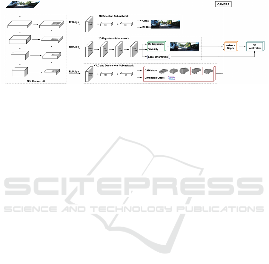
Figure 2: An overview of our monocular 3D detection architecture (text best viewed in zoom). We start with a universal

backbone network (Mask R-CNN (He et al., 2017)) and complement it with three sub-networks: 2D object detection sub-

network, 2D keypoints regression sub-network, and dimension regression sub-network. The network is trained end-to-end

using a multi-task loss function.

2D Object Detection. For 2D detection, we fol-

low the original Mask R-CNN architecture (He et al.,

2017), which includes Feature Pyramid Network

(FPN) (Lin et al., 2017a), Region Proposal Network

(RPN) (Ren et al., 2015) and RoIAlign module (He

et al., 2017). The RPN generates 2D anchor-boxes

with a set of ﬁxed aspect ratios and scales through-

out the area of the provided feature maps, which are

scored for the presence of the object of interest and

adjusted. The spatial diversity of the proposed loca-

tions is processed by the RoIAlign block, converting

each feature map, framed by the region of interest,

into a ﬁxed-size grid, preserving an accurate spatial

location through bilinear interpolation. Followed by

fully connected layers, the network splits into two fea-

ture sharing branches for the bounding box regression

and object classiﬁcation. During training, we utilize a

sum of smooth L

and cross-entropy loss for each task

respectively as our 2D detection loss L

, as proposed

by (Ren et al., 2015). Though we do not directly uti-

lize the predicted 2D bounding boxes, we have exper-

imentally observed the 2D detection sub-network to

stabilize training.

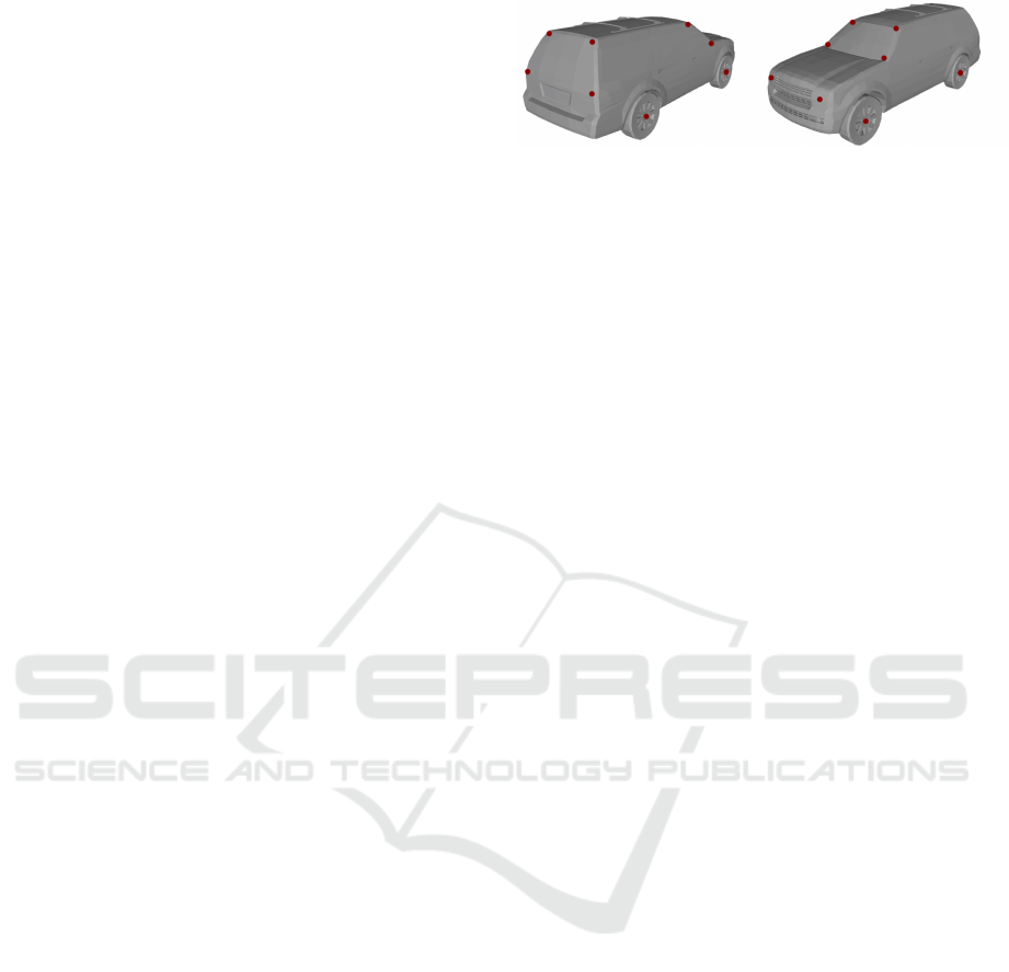
2D Keypoint Detection. As described in greater

detail in Section 4.1, we have created keypoint an-

notations for object instances encountered in the im-

ages of our training set (see Figure 3 and its caption

for the details on our choice of the keypoints). Thus,

using our 2D object detection sub-network, we learn

to predict coordinates k

(x,y)

= (x

) and a visibil-

ity state v

for each of the manually-chosen 14 key-

points K = {(x

)

k=1

}. Unlike suggested in (He

et al., 2017; Tompson et al., 2014), we directly regress

onto 2D coordinates of keypoints. The visibility state,

determined by the occlusion and truncation of an in-

stance, is a binary variable, and no difference between

occluded, self-occluded and truncated states is made.

Producing visibility estimates helps propagate infor-

mation during training for visible keypoints only and

acts as an auxiliary supervision for orientation sub-

network. During training, similar to our 2D object de-

tection sub-network, we minimize the multi-task loss

combining smooth L

loss for coordinates regression

and cross-entropy loss for visibility state classiﬁca-

tion, deﬁned as:

coord

∑

k=1

· L

smooth



(x,y)

pred

(x,y)



vis

= −

∑

k=1

logv

pred

= L

coord

+ L

vis

(1)

where 1

is the visibility indicator of k-th keypoint,

while k

(x,y)

and k

pred

(x,y)

denote ground-truth and pre-

dicted 2D coordinates, normalized and deﬁned in a

reference frame of a speciﬁc feature map post RoI-

alignment. Similarly, v

is the ground truth visibil-

ity status, while v

pred

is the estimated probability that

keypoint k is visible.

3D Dimension Estimation and Geometric Clas-

siﬁcation. To each annotated 3D instance in the

dataset, we have assigned a 3D CAD model out of

a predeﬁned set of 5 templates, obtaining 5 distinct

geometric classes of instances. The assignment has

been made based on the width, length and height ra-

tios only. For each geometric class, we have com-

puted mean dimensions (µ

,µ

) over all assigned

annotated 3D instances.

During training the 3D dimension estimation and

geometric class selection sub-network, we utilize a

multi-task loss combining cross-entropy loss (for the

VISAPP 2020 - 15th International Conference on Computer Vision Theory and Applications

654

geometric class selection) and a smooth L

loss for

dimension regression. Instead of regressing the abso-

lute dimensions, we predict the differences D

offset

(∆w,∆h,∆l) = (w − µ

,h − µ

,l − µ

) from the mean

dimensions in the log-space:

dim

= smooth



log(D

offset

− D

pred

offset

)



, (2)

where D

offset

and D

pred

offset

represent the ground-truth

and predicted offsets to the class mean values along

each dimension, respectively.

Reasoning about Instance Depth. We deﬁne in-

stance depth as the depth Z of a vertical plane pass-

ing through the two closest of visible keypoints, de-

ﬁned in the camera reference frame. To compute this

depth value, we use predicted 2D keypoints (x

)

and (x

), instance height h (in meters), and its ge-

ometric class. First, we select two keypoints (x

)

and (x

) detected in the image and compute their

y-difference h

= |y

− y

|. We then select the corre-

sponding two keypoints (x

cad

) and (x

cad

) in

3D CAD model reference frame and compute their

height ratio r

cad

= y

cad

. Finally, the distance

to the object Z is deﬁned from the pinhole camera

model:

Z = f ·

cad

· h

, (3)

where f is a focal length of the camera, known for

each frame. Figire 1 illustrates this computation.

Depth coordinate Z allows to retrieve the remaining

3D location coordinates of one of the selected key-

points, using the back-projection mapping:

X = Z ·

{1,2}

− p

, Y = Z ·

{1,2}

− p

, (4)

giving predictions k

pred

(X,Y,Z)

= (X

),k ∈ {1,2},

where (p

, p

) are the camera principal point coordi-

nates in pixels and (x

) and (x

) are predicted

2D keypoints.

In this computation, we use the two closest of de-

tected visible keypoints, which commonly results in

selecting keypoints physically located at instance cor-

ners. We note that this step is crucial to the success

of our method, as, if no keypoints are visible on the

instance, we fail to recover its depth and precisely lo-

calize it (even though it may not be entirely occluded).

Orientation Estimation. Direct estimation of ori-

entation R in a camera reference frame is not feasible,

as the region proposal network propagates the con-

text within the crops solely, cutting off the relation of

the crop to the image plane. Inspired by (Mousavian

et al., 2017), we represent the global orientation as a

combination of two rotations with azimuths deﬁned

as:

θ = θ

loc

+ θ

ray

, (5)

where θ

loc

is the object’s local orientation within the

region of interest, and θ

ray

is a ray direction from

the camera to the object center, directly found from

the 3D location coordinates. We estimate θ

loc

using

a modiﬁcation of the MultiBin approach (Mousavian

et al., 2017). Speciﬁcally, instead of splitting the ob-

jective into angle conﬁdence and localization parts,

we discretize the angle range from 0

◦

to 360

◦

degrees

into 72 non-overlapping bins and compute the proba-

bility distribution over this set of angles by a softmax

layer. We train the local orientation sub-network us-

ing cross-entropy as a loss function. To obtain the

ﬁnal prediction for θ

loc

, we utilize the weighted mean

of the bins medians (W M(θ

loc

)), adopting the softmax

output as the weights. Given 3D location coordinates

(X,Z) of one of the keypoints and the weighted mean

local orientation W M(θ

loc

), the global orientation is:

θ = W M(θ

loc

) + arctan





. (6)

3D Object Detection. To obtain the center C of

the ﬁnal 3D bounding box, we use the global ori-

entation R and the distance between the keypoint

and the object center. For a particular CAD model,

given the weight, height and length ratio between

the selected keypoint and the object center r

cad

) estimated object di-

mensions D and global orientation R, the location C

is predicted as

C = (X,Y,Z) ± R · D  r

cad

, (7)

where  stands for an element-wise product. Depend-

ing on the selected keypoint position (left or right,

etc.), a sign is chosen for each dimension.

Multi-head Reprojection Consistency Loss. One

approach when training the system would be to opti-

mize a sum of losses suffered by individual compo-

nents:

L = L

+ L

dim

+ L

ori

. (8)

However, while each sub-network is independent of

its neighbors and unaware of other predictions, its ge-

ometric components are strongly interrelated. To pro-

vide consistency between the network branches, we

introduce a loss function which integrates all the pre-

dictions. Predicted 3D keypoint coordinates k

pred

(X,Y,Z)

in a CAD model coordinate frame are scaled using

D, rotated using R, translated using C, and back-

projected into the image plane via camera projection

matrix to obtain 2D keypoint coordinates k

pred+proj

(x,y)

Monocular 3D Object Detection via Geometric Reasoning on Keypoints

655

Project(k

pred

(X,Y,Z)

). A similar approach is applied to the

eight corners K

of the 3D bounding box obtained

from 3D detection and orientation estimates, to ensure

that they ﬁt tightly into the ground truth 2D bounding

box after back-projection. This leads us to adding the

reprojection consistency loss L

repro

to the ﬁnal opti-

mization:

repro

∑

k∈K∪K

smooth



pred+proj

(x,y)

− k

(x,y)



L = L

+ L

dim

+ L

ori

+ L

repro

(9)

4 EXPERIMENTS

4.1 Dataset Annotation

We train and evaluate our approach using the KITTI

3D object detection benchmark dataset, selecting only

objects of class “car”. For the sake of comparison

with state-of-the-art methods, we follow the setup

presented in (Chen et al., 2016), which provides 3712

and 3769 images for training and validation, respec-

tively, along with the camera calibration data. To

extend KITTI dataset with assignment of geometric

classes using CAD models and keypoints 2D coordi-

nates, we employ the approach and data provided in

(Xiang et al., 2015). Depending on the ratios between

height, length and width, each car instance is associ-

ated with one of ﬁve 3D CAD model classes from a

predeﬁned set of CAD templates, presented on Fig-

ure 2. We manually annotated each CAD model with

14 keypoint locations, ending up with a total human

labour of 70 annotations in the entire dataset. Fig-

ure 3 displays an example of the annotated keypoints,

most of which are a common choice (Everingham

et al., 2010) due to their interpretability, such as the

car’s edges, carcass, etc.; we also included corners of

windshields to deal with the height of each instance.

To obtain 2D coordinates of the keypoints, we back-

projected CAD models from 3D space to the image

plane using ground truth location, dimension and ro-

tation values. Simultaneous projection of all 3D CAD

models on a scene provides us with a depth ordering

mask, allowing for deﬁning the visibility state of each

keypoint.

4.2 Experimental Setup

Network Architecture. We utilize Mask R-CNN

with a Feature Pyramid Network (Lin et al., 2017a),

based on a ResNet-101 (He et al., 2016) as our back-

bone network for the multi-level feature extraction.

Instead of the higher resolution 14 × 14 and 28 × 28

Figure 3: An example of our annotation of 3D keypoints.

We label 4 centers of wheels, 8 corners of front and back

windshields per each, and 2 centers of headlights. Per each

3D CAD model, we form the annotation so as to ensure that

the two keypoints on each of the windshields form near-

vertical lines.

feature maps in the original architecture, we stack the

same amount of 3×3 kernels, followed by a fully con-

nected layer to predict 2D normalized coordinates and

visibility states for each of the 14 keypoints. From the

same feature maps, we branch a fully-connected layer

predicting local orientation in bins of 5

◦

each, total-

ing 72 output units. The feature sharing between key-

points and local orientation was found crucial for net-

work performance, as both characteristics imply sim-

ilar geometric reasoning. In parallel to 2D detection

and 2D keypoints estimation, we create a sub-network

of a similar architecture for dimension regression and

classiﬁcation into geometric classes. The remaining

components, including RPN, RoIAlign, bounding box

regression and classiﬁcation heads, are implemented

following the original Mask R-CNN design. For in-

stance depth retrieval we use only four pairs of key-

points: corners of the front and rear windows. Other

keypoints are used for additional supervision in con-

sistency loss calculation during training.

Model Optimization Details. We set hyperparam-

eters following Mask R-CNN work (He et al., 2017).

The RPN anchor set covers ﬁve scales, adjusting them

to the values of 4, 8, 16, 32, 64, and three default

aspect ratios. Each mini-batch consists of 2 images,

producing 256 regions of interest, with a positive to

negative samples ratio set 1:3, to achieve class sam-

pling balance during training. Any geometric aug-

mentations over the images are omitted, solely ap-

plying image padding to meet the network architec-

ture requirements. ResNet-101 is initialized with the

weights pre-trained on Imagenet (Deng et al., 2009),

and frozen during further training steps. We ﬁrst

train the 2D detection and classiﬁcation sub-network

for 100K iterations, adopting Adam optimizer with

a learning rate of 10

−4

throughout the training, set-

ting weight decay of 0.001 and momentum of 0.9.

Then 2D keypoints and local orientation are trained

for 50K iterations. Finally, enabling the multi-head

consistency loss, the whole network is trained in an

end-to-end fashion for 50K iterations. We combine

VISAPP 2020 - 15th International Conference on Computer Vision Theory and Applications

656

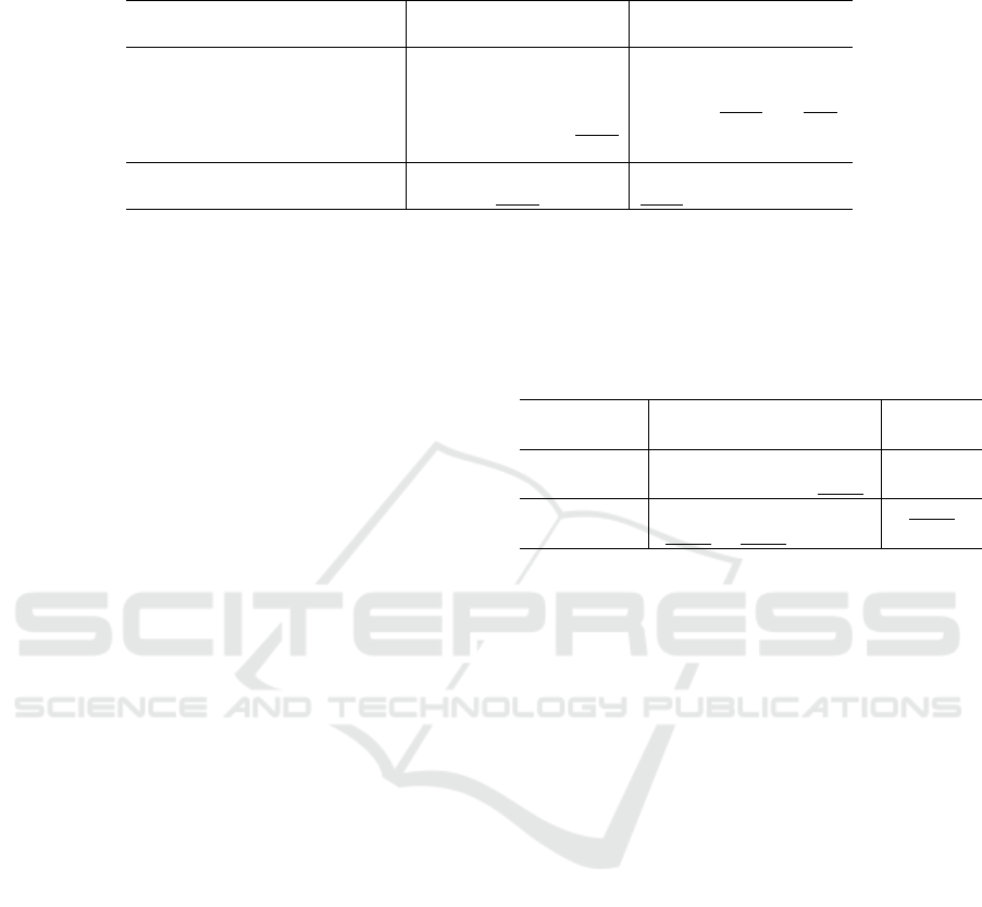
Table 1: 3D detection performance: Average Precision of 3D bounding boxes on KITTI val set. The best score is in bold,

the second best underlined. Ours (+loss) indicates a base network setup, trained with a consistency reprojection loss.

Method

IoU = 0.5 IoU = 0.7

Easy Moderate Hard Easy Moderate Hard

Mono3D (Chen et al., 2016) 25.19 18.20 15.52 2.53 2.31 2.31

OFT-Net (Roddick et al., 2018) - - - 4.07 3.27 3.29

MonoGRNet (Qin et al., 2019) 50.51 36.97 30.82 13.88 10.19 7.62

MF3D (Xu and Chen, 2018) 47.88 29.48 26.44 10.53 5.69 5.39

MonoDIS (Simonelli et al., 2019) - - - 18.05 14.98 13.42

Ours 48.81 30.17 20.07 11.91 6.64 4.28

Ours (+loss) 50.82 31.28 20.21 13.96 7.37 4.54

losses from all of the network outputs, weighting

them equally.

Evaluation Metrics. We evaluate the network un-

der the conventional KITTI benchmark protocol,

which enables comparison across approaches. Car

category is the sole subject of our focus. By de-

fault, KITTI settings require evaluation in 3 regimes:

easy, moderate and hard, depending on the instance

difﬁculty of a potential detection. 3D bounding box

detection performance implies 3D Average Precision

(AP3D) evaluation, setting Intersection over Union

(IoU) threshold to 0.5 and 0.7.

4.3 Experimental Results

3D Object Detection. We compare the perfor-

mance with 5 monocular 3D object detection meth-

ods: Mono3D (Chen et al., 2016), OFT-Net (Roddick

et al., 2018), MonoGRNet (Qin et al., 2019), MF3D

(Xu and Chen, 2018), and MonoDIS (Simonelli et al.,

2019), which reported their results on the same vali-

dation set for the car class. We borrow the presented

average precision numbers from their published re-

sults. The results are reported in Table 1. The ex-

periments show that our approach outperforms state-

of-the-art methods on the easy subset by a small mar-

gin while remaining the second best on the moderate

subset. This observation aligns with our intuition that

visible salient features such as keypoints are crucial

to the success of 3D pose estimation. For the moder-

ate and hard images, 2D keypoints are challenging to

robustly detect due to the high occlusion level or the

low resolution of the instance. We also measure the

effect of the reprojection consistency loss on our net-

work performance, observing a positive effect of our

loss function.

3D Bounding Box and Global Orientation Estima-

tion. We follow the experiment presented in (Qin

et al., 2019), evaluating the quality of the 3D bound-

ing boxes sizes estimation, as well as the orientation

in a camera coordinate system. We present our mean

errors along with those of (Qin et al., 2019; Chen

et al., 2016), borrowed from their work, in Table 2.

Table 2: 3D bounding box and orientation mean errors:

The best score is in bold, the second best underlined.

Method

Size (m)

Ori. (rad)

Height Width Length

Mono3D 0.172 0.103 0.504 0.558

MonoGRNet 0.084 0.084 0.412 0.31

Ours 0.115 0.107 0.516 0.215

Ours (+loss) 0.101 0.091 0.403 0.191

Though, the sizes of the 3D bounding boxes do not

differ severely among the approaches, due to the es-

timating the offset from the median bounding box,

the orientation estimation results differ signiﬁcantly.

Since we retrieve global orientation via geometric

reasoning, learning local orientation from 2D image

features, the network provides more accurate predic-

tions, in contrast to obtaining orientation from the re-

gressed 3D bounding box corners.

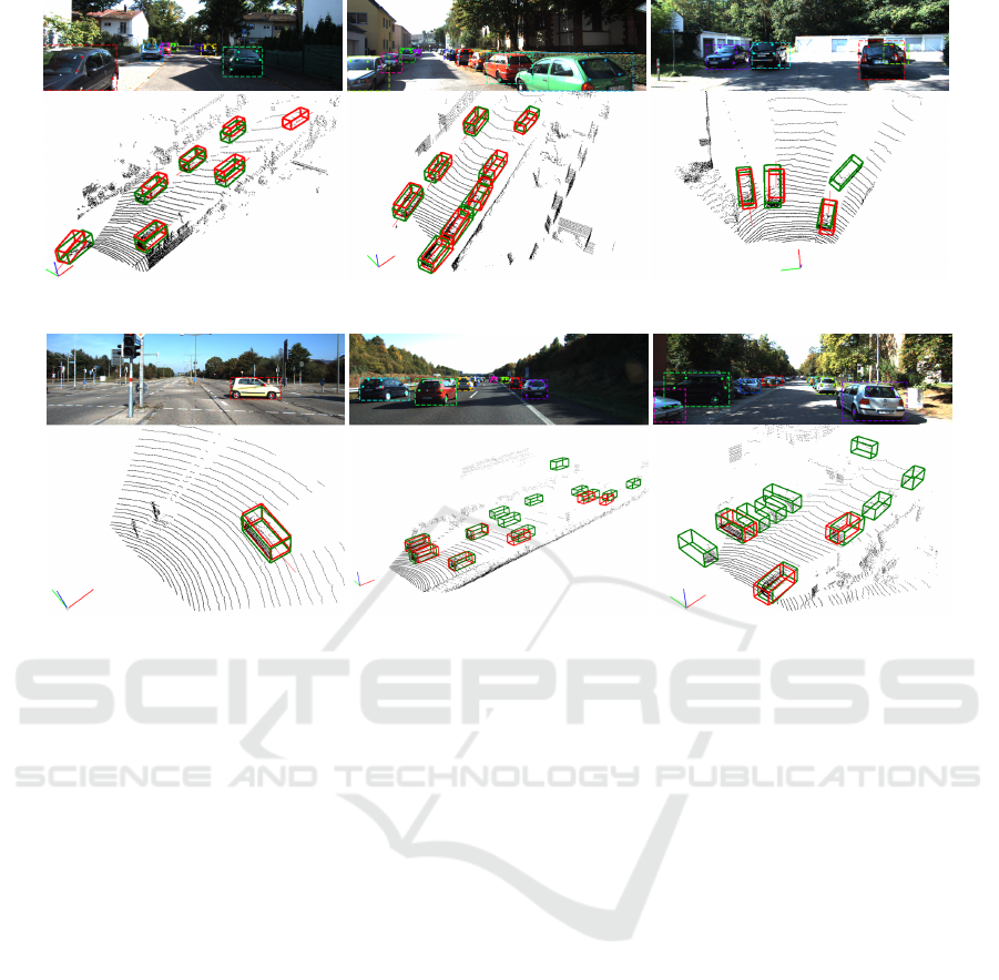
Qualitative Results. We provide a qualitative illus-

tration of the network performance in Figure 4, dis-

playing six road scenes with distinct levels of difﬁ-

culty. In typical cases, our approach produces ac-

curate 3D bounding boxes for all instances, along

with the global orientation and 3D location. Remark-

ably, the truncated objects can also be successfully

detected, given that only one pair of keypoints hits

the image. Some hard cases, i.e. (e) and (f), primarily

consist of objects that are distant, highly occluded or

even invisible on the image. We believe such failure

cases to be a common limitation of monocular image

processing methods.

5 CONCLUSIONS

In this work, we presented a novel deep learning-

based framework for monocular 3D object detection

Monocular 3D Object Detection via Geometric Reasoning on Keypoints

657

(a) (b) (c)

(d) (e) (f)

Figure 4: Qualitative results. The upper part of each sub-ﬁgure contains 2D detection inference, including 2D bounding and

2D locations of the visible keypoints. Each instance and its keypoints are displayed their distinctive color. The lower part

visualizes the 3D point cloud, showing the camera location as the colored XYZ axes. Green and red colors stand for the

ground truth and predicted 3D bounding boxes respectively. The scenes were selected to express diversity in complexity and

cars positioning w.r.t. the camera.

combining well-known detectors with geometric rea-

soning on keypoints. We proposed to estimate cor-

respondences between the detected 2D keypoints and

their 3D counterparts annotated on the surface of 3D

CAD models to solve the object localization prob-

lem. Results of the experimental evaluation of our ap-

proach on the subsets of the KITTI 3D object detec-

tion benchmark demonstrate that it outperforms the

competing state-of-the-art approaches when the tar-

get objects are clearly visible, leading us to hypothe-

size that dense depth estimation is redundant for 3D

detection in some instances. We have demonstrated

our multi-task reprojection consistency loss to signif-

icantly improve performance, in particular, the orien-

tation of detections.

ACKNOWLEDGEMENT

E. Burnaev and A. Artemov were supported by the

Russian Science Foundation Grant 19-41-04109.

REFERENCES

Chabot, F., Chaouch, M., Rabarisoa, J., Teuli

ere, C., and

Chateau, T. (2017). Deep manta: A coarse-to-ﬁne

many-task network for joint 2d and 3d vehicle analysis

from monocular image. In CVPR, pages 2040–2049.

Chen, X., Kundu, K., Zhang, Z., Ma, H., Fidler, S., and

Urtasun, R. (2016). Monocular 3d object detection

for autonomous driving. In CVPR, pages 2147–2156.

Chen, X., Ma, H., Wan, J., Li, B., and Xia, T. (2017). Multi-

view 3d object detection network for autonomous

driving. In CVPR, pages 1907–1915.

Deng, J., Dong, W., Socher, R., Li, L.-J., Li, K., and Fei-

Fei, L. (2009). Imagenet: A large-scale hierarchical

image database. In CVPR, pages 248–255. Ieee.

Everingham, M., Van Gool, L., Williams, C. K., Winn, J.,

and Zisserman, A. (2010). The pascal visual object

classes (voc) challenge. IJCV, 88(2):303–338.

Geiger, A., Lenz, P., Stiller, C., and Urtasun, R. (2013).

Vision meets robotics: The kitti dataset. IJRR,

32(11):1231–1237.

Geiger, A., Lenz, P., and Urtasun, R. (2012). Are we ready

for autonomous driving? the kitti vision benchmark

suite. In CVPR, pages 3354–3361. IEEE.

VISAPP 2020 - 15th International Conference on Computer Vision Theory and Applications

658

Godard, C., Mac Aodha, O., and Brostow, G. J. (2017). Un-

supervised monocular depth estimation with left-right

consistency. In CVPR, pages 270–279.

He, K., Gkioxari, G., Doll

ar, P., and Girshick, R. (2017).

Mask r-cnn. In ICCV, pages 2961–2969.

He, K., Zhang, X., Ren, S., and Sun, J. (2016). Deep resid-

ual learning for image recognition. In CVPR, pages

770–778.

Hejrati, M. and Ramanan, D. (2012). Analyzing 3d objects

in cluttered images. In NIPS, pages 593–601.

Ku, J., Moziﬁan, M., Lee, J., Harakeh, A., and Waslander,

S. L. (2018). Joint 3d proposal generation and object

detection from view aggregation. In IROS, pages 1–8.

IEEE.

Lang, A. H., Vora, S., Caesar, H., Zhou, L., Yang, J., and

Beijbom, O. (2019). Pointpillars: Fast encoders for

object detection from point clouds. In CVPR, pages

12697–12705.

Lin, T.-Y., Doll

ar, P., Girshick, R., He, K., Hariharan, B.,

and Belongie, S. (2017a). Feature pyramid networks

for object detection. In CVPR, pages 2117–2125.

Lin, T.-Y., Goyal, P., Girshick, R., He, K., and Doll

ar, P.

(2017b). Focal loss for dense object detection. In

ICCV, pages 2980–2988.

Liu, S., Qi, L., Qin, H., Shi, J., and Jia, J. (2018). Path

aggregation network for instance segmentation. In

CVPR, pages 8759–8768.

Liu, W., Anguelov, D., Erhan, D., Szegedy, C., Reed, S.,

Fu, C.-Y., and Berg, A. C. (2016). Ssd: Single shot

multibox detector. In ECCV, pages 21–37. Springer.

Martinez, J., Hossain, R., Romero, J., and Little, J. J.

(2017). A simple yet effective baseline for 3d human

pose estimation. In ICCV, pages 2640–2649.

Mehta, D., Rhodin, H., Casas, D., Fua, P., Sotnychenko,

O., Xu, W., and Theobalt, C. (2017a). Monocular 3d

human pose estimation in the wild using improved cnn

supervision. In 3DV, pages 506–516. IEEE.

Mehta, D., Sridhar, S., Sotnychenko, O., Rhodin, H.,

Shaﬁei, M., Seidel, H.-P., Xu, W., Casas, D., and

Theobalt, C. (2017b). Vnect: Real-time 3d human

pose estimation with a single rgb camera. ACM ToG,

36(4):44.

Mousavian, A., Anguelov, D., Flynn, J., and Kosecka, J.

(2017). 3d bounding box estimation using deep learn-

ing and geometry. In CVPR, pages 7074–7082.

Qin, Z., Wang, J., and Lu, Y. (2019). Monogrnet: A ge-

ometric reasoning network for monocular 3d object

localization. In AAAI, volume 33, pages 8851–8858.

Ramakrishna, V., Kanade, T., and Sheikh, Y. (2012). Recon-

structing 3d human pose from 2d image landmarks. In

ECCV, pages 573–586. Springer.

Redmon, J., Divvala, S., Girshick, R., and Farhadi, A.

(2016). You only look once: Uniﬁed, real-time ob-

ject detection. In CVPR, pages 779–788.

Ren, S., He, K., Girshick, R., and Sun, J. (2015). Faster

r-cnn: Towards real-time object detection with region

proposal networks. In NIPS, pages 91–99.

Roddick, T., Kendall, A., and Cipolla, R. (2018). Ortho-

graphic feature transform for monocular 3d object de-

tection. arXiv preprint arXiv:1811.08188.

Simonelli, A., Bul

o, S. R. R., Porzi, L., L

opez-Antequera,

M., and Kontschieder, P. (2019). Disentangling

monocular 3d object detection. arXiv preprint

arXiv:1905.12365.

Tompson, J. J., Jain, A., LeCun, Y., and Bregler, C. (2014).

Joint training of a convolutional network and a graph-

ical model for human pose estimation. In NIPS, pages

1799–1807.

Wu, J., Xue, T., Lim, J. J., Tian, Y., Tenenbaum, J. B.,

Torralba, A., and Freeman, W. T. (2016). Single im-

age 3d interpreter network. In ECCV, pages 365–382.

Springer.

Xiang, Y., Choi, W., Lin, Y., and Savarese, S. (2015). Data-

driven 3d voxel patterns for object category recogni-

tion. In ICCV.

Xu, B. and Chen, Z. (2018). Multi-level fusion based 3d

object detection from monocular images. In CVPR,

pages 2345–2353.

Yan, Y., Mao, Y., and Li, B. (2018). Second:

Sparsely embedded convolutional detection. Sensors,

18(10):3337.

Yang, B., Luo, W., and Urtasun, R. (2018). Pixor: Real-

time 3d object detection from point clouds. In CVPR,

pages 7652–7660.

Zhou, Y. and Tuzel, O. (2018). Voxelnet: End-to-end learn-

ing for point cloud based 3d object detection. In

CVPR, pages 4490–4499.

Monocular 3D Object Detection via Geometric Reasoning on Keypoints

659