Image-based Classification of Swiss Traditional Costumes using
Contextual Features
Artem Khatchatourov and Christoph Stamm
Institute of Mobile and Distributed Systems, FHNW University of Applied Sciences and Arts Northwestern Switzerland,
Bahnhofstrasse 6, 5210 Windisch, Switzerland
Keywords:
Feature-based Object Recognition, Pattern Matching, Clothing Recognition, Machine Learning.
Abstract:
In this work we propose a method for feature-based clothing recognition, and prove its applicability by per-
forming image-based recognition of Swiss traditional costumes. We employ an estimation of a simplified
human skeleton (a poselet) to extract visually indistinguishable but reproducible features. The descriptors
of those features are constructed, while accounting for possible displacement of clothes along human body.
The similarity metrics mean squared error and correlation coefficient are surveyed, and color spaces YIQ and
CIELAB are investigated for their ability to isolate scene brightness in a separate channel. We show that the
model trained with mean squared error performs best in the CIELAB color space and achieves an F
0.5
-score of
0.77. Furthermore, we show that omission of the brightness channel produces less biased, but overall poorer
descriptors.
1 INTRODUCTION
Traditionally, feature-based object recognition is ac-
complished by learning features of an object and
matching them to those extracted from a new im-
age. The most well-known example of this method
is the work of Lowe et al. (Lowe, 1999), which de-
scribes the Scale-Invariant Feature Transform method
(SIFT). In general, this approach only works on mass-
produced and rigid objects that look exactly alike in
every picture. Feature-based object recognition will
fail to recognize flexible objects, as they produce vi-
sual features that are irreproducible in other images.
Therefore, in this work, instead of visual keypoints
we use contextual ones, defined by a simplified ap-
proximation of human skeleton, called poselet. Even
though human features are concealed under clothes,
newly developed methods for pose estimation allow
to extract them from the image.
Another drawback of established feature-based
object recognition methods is their color-blindness.
Most of them are constrained to work only with
gray-scale images in order to maximize invariance to
changing lighting conditions between the scenes. For
clothing recognition, however, color is an essential
feature that must be included in the feature descrip-
tion. The influence of illumination in the image can
be mitigated by isolating the brightness information
to a luminance channel in the color spaces YIQ and
CIELAB.
In the next section of this work we explore state-
of-the-art methods for object and clothing recogni-
tion. In Section 3 we introduce the Swiss traditional
costume dataset and describe our approach for feature
extraction. We propose a matching method and con-
struct feature descriptors in Section 4. In Section 5
we discuss the conducted experiments and determine
optimal parameters for maximizing prediction preci-
sion. Finally, conclusions are drawn in Section 6.
2 RELATED WORK
The task of garment recognition in images was tack-
led by Yamaguchi et al. (Yamaguchi et al., 2012) and
by Kalantidis et al. (Kalantidis et al., 2013). Both
works use image segmentation and pose estimation to
identify spacial location of a certain region on the hu-
man body. Combining the position and shape of this
region with information of the neighboring regions
enables its classification as a specific clothing item.
Additionally, color histograms were introduced to de-
termine the color of a garment. Both of these works
use the Fashionista dataset introduced previously (Ya-
maguchi et al., 2012) containing 158,235 images of
people wearing common, every-day clothes. Garment
412
Khatchatourov, A. and Stamm, C.
Image-based Classification of Swiss Traditional Costumes using Contextual Features.
DOI: 10.5220/0009102404120420
In Proceedings of the 15th International Joint Conference on Computer Vision, Imaging and Computer Graphics Theory and Applications (VISIGRAPP 2020) - Volume 4: VISAPP, pages
412-420
ISBN: 978-989-758-402-2; ISSN: 2184-4321
Copyright
c
 2022 by SCITEPRESS – Science and Technology Publications, Lda. All rights reserved

items in each image are marked with a polygon and
annotated. Another clothing dataset, DeepFashion,
introduced in (Liu et al., 2016) contains over 800,000
images. In contrast, our Swiss traditional costume
dataset contains 247 classes and merely 1540 samples
overall.
In cases where no large dataset is available, we
use feature recognition to find objects from a train-
ing set as small as a single sample. Generally, it only
works well with non-deformable objects that look ex-
actly alike on all images, which is almost impossible
to achieve with clothing. Nevertheless, feature based
garment recognition has been attempted in numerous
works. Most notably, Chen et al. (Chen et al., 2012)
use the work in (Eichner et al., 2012) to locate body
parts, Maximum Response Filters (Varma and Zisser-
man, 2005) to describe texture and color in LAB color
space. Additionally, dense SIFT features along the
body are used to describe the garment on each body
part (Lowe, 1999).
3 TRADITIONAL COSTUMES
Traditional costumes are a special kind of clothing
used to represent culture and customs of a community.
The costume is bound to a specific region. In Switzer-
land, the sizes of such regions vary from a whole can-
ton (administrative subdivision of Switzerland) to an
area as small as single village. People from every re-
gion incorporate their traditions, values and history
into costumes complementing them with distinctive
accessories and details. Such celebratory costumes
are often worn at inter-regional festivities to represent
heritage of a particular locality.
Additionally to celebratory costumes, regions or
groups of regions define their own costumes for other
purposes. Work wear is usually common for each can-
ton spanning many regions. Also, most protestant re-
gions often define special clothing for church visits.
Some regions and cantons have their own costumes
for certain traditional professions like wine or cheese
makers. The aim of this project is to help experts and
amateurs to identify the costumes, which is usually
not possible without proper reference material.
A special committee in every canton defines regu-
lations for a costume’s appearance in a written form,
and sets up guidelines that every tailor must follow.
Once set, these guidelines do not change. Many cos-
tumes, however, allow for some variations: e.g. a
different set of colors for certain clothing parts or a
winter version of a costume for cold weather.
Figure 1: Distribution of samples among the 100 largest
subtypes. The amount of samples of each body part is
marked with color.
3.1 Dataset
Costume descriptions are written in the official lan-
guage of a given canton: German, French, Italian or
even Romansh; and contain many specific names for
clothing parts. The task of teaching a computer to
deduce a visual image from these descriptions seems
to be infeasible. Thus, it was decided to collect a
dataset of images. Each image in this dataset depicts
one person wearing a traditional costume. In cases
where variations of a costume are defined, we create
subtypes of this costume. We allow only one level
of subtype for a costume supertype. Subtypes are
used only to produce consistent descriptors, the clas-
sification goal, however, remains supertype classifi-
cation. Ultimately, our dataset contains 1540 images
from 274 supertypes and 427 subtypes. The small
size of the dataset correlates with the small number
of unique costume samples available. The national
costume community is very small and each costume
is tailored to its owner. To our knowledge, this the
first attempt to apply machine learning to recognize
traditional clothing.
We have decided against dataset augmentation be-
cause of the several reasons: 1. linear transformation
is reverted in the preprocessing stage; 2. non-linear
transformation distorts important patterns on the cos-
tume; 3. altering color and adding noise to images in-
terferes with pattern alignment at learning stage. This
dataset defines the ground truth of costume appear-
ance in our work. The images are distributed non-
uniformly among classes as shown in Figure 1. The
amount of samples per costume type is very unbal-
anced. Usually, the prevalence of a costume in the
dataset is proportional to the population of its region
of origin, but some of the smaller classes result from
fracturing the costume supertype.
Image-based Classification of Swiss Traditional Costumes using Contextual Features
413

3.2 Preprocessing
As we have seen in the works in Section 2, it is im-
portant to determine the pose of a person in the image.
We accomplish this using the open-source OpenPose
library (Cao et al., 2018). It is based on the work of
Wei et al. (Wei et al., 2016), who uses deep learn-
ing to estimate the location of body parts in the im-
age and connects best fitting parts together to produce
a poselet: a simplified human skeleton that approxi-
mates a pose. This technique was further improved
by the work of Cao et al. (Cao et al., 2017), who
introduced affinity fields for better handling of multi-
person scenes.
We use OpenPose with the BODY25 model for
poselet detection, which produces a poselet with 25
keypoints, numbered as shown in Figure 2a. In most
cases the approximations are correct, however, Open-
Pose sometimes fails to properly locate legs con-
cealed by a skirt or a dress as seen in Figure 2b. It
can also be misled by unusual shapes of some cloth-
ing parts, as shown in Figure 2c. In this example, the
elbow keypoints are placed onto balloon-sleeves. As
a consequence, the attached hand keypoints are mis-
placed as well. Poselet parts from incorrectly recog-
nized keypoints must be filtered from the training set
manually.
We identify twelve poselet connections, marked
red in Figure 2a, where we expect to find clothing
parts. From each connection we cut out a rectangu-
lar image patch, rotated in alignment with this con-
nection. The use of patches between two keypoints
as features removes the variance in rotation and scale.
We proceed by mirroring the opposing patches. This
is possible due to the symmetry of costumes. Mirror-
ing reduces the number of features for each class from
twelve to six. At the same time, it doubles the amount
of patches for each feature and, thus, mitigates the
scarcity of samples in the dataset.
4 DESCRIPTOR CONSTRUCTION
Our goal is to produce a general description for each
feature, meaning that it must resemble all possible
patches equally well. Ideally, such a description
should be computed by acquiring mean pixel inten-
sities of all patches. In our case this approach is not
sufficient, since there is always a certain shift among
the patch contents caused by variation in camera an-
gle and fit of clothes. Our strategy is to allow for some
transformation of patches and combine them at a lo-
cation where they are the most similar.
We denote a patch collection C = {c
1
,c
2
,...,c
n
},
22
23
24
19
20
21
17
15
18
16
0
12
torso
135x57
13
hip
105x45
9
4
3
7
elbow
75x33
6
arm
75x33
5
shoulder
45x21
1 2
8
14
thigh
105x45
10
11
(a) (b) (c)
Figure 2: Pose estimation with BODY25 model: a) posi-
tions of poselet joints, indexes and patch sizes (in pixels)
used in our work; demonstration of misplaced positions of
b) a leg and c) an elbow in the poselet.
which contains n patches of the same feature, orig-
inating from the same subtype of costume. The
patches in the collection are compared in pairs and the
pair which appears to be most similar is merged pro-
ducing a new patch. In the next iteration, this patch is
compared to the remaining patches in the collection,
and, again, the most similar pair is combined. Note,
that there is no need to recalculate the pairs that have
not been merged in the previous iteration. This pro-
cess is repeated until all patches have been merged
into one. This last patch is the feature descriptor f .
For each pair of patches we denote a target patch t
and a query patch q, where t,q ∈C. The query patch is
displaced relative to the target patch by ¯x, ¯y and rota-
tion α. The best position to merge them is where they
are most similar. For similarity ρ(t,q) between the
two patches we evaluate two different metrics: mean
squared error (mse) and correlation coefficient (r). We
will cover both metrics in detail in Section 4.5.
4.1 Displacement
The similartiy of a patch pair is calculated by iterating
through every pixel x and y in t, and their counterparts
x
0
and y
0
in q, for every displacement ¯x, ¯y and α. For
convenience, we denote the displacement parameters
ξ, thus:
ξ = ( ¯x, ¯y,α). (1)
Our goal is to determine the displacement position
where mse is minimal or r is maximal, depending on
the metric used:
ρ(t,q) =





argmin
ξ
mse
ξ
(t,q)
argmax
ξ
r
ξ
(t,q)
(2)
We limit the displacement to 1/4 of the width and
height of a target patch, and rotation of −10
◦
to 10
◦
VISAPP 2020 - 15th International Conference on Computer Vision Theory and Applications
414

d
h'
w'
h
w
α
γ
Figure 3: Rotating the patch of size h × w by α extends
its bounding box (dashed lines) to new dimensions h
0
× w
0
.
Note that the length of the hypotenuse stays unchanged,
while its angle to w
0
varies.
with a step of 2
◦
. Our experiments have shown that al-
lowing for larger displacement enables the algorithm
to achieve maximal similarity by reducing the over-
lap area of the two patches to a minimum instead of
matching the patterns.
4.2 Displacement Calculation
Mapping of every pixel (x,y) in q to its transformed
position (x
0
,y
0
) in t is accomplished by rotating of q
by α, translating it by ¯x and ¯y and compensating the
size differences of the two patches, which gives us the
following equation:


x
0
y
0
1


= M
ξ


x
y
1


. (3)
The affine transformation matrix M is computed from
five separate matrices as follows:
M
ξ
= T
D
T
∆
T
o
+
RT
o
−
, (4)
where T
o
+
translates the center (ˆx
q
, ˆy
q
) of q to the ori-
gin (coordinates (0,0)), R rotates the image around
the origin by α, and T
o
−
returns the center of q to the
original position:
T
o
+/−
=


1 0
+/−
ˆx
q
0 1
+/−
ˆy
q
0 0 1


,R =


cosα sinα 0
−sinα cosα 0
0 0 1


.
(5)
After rotation the patch is translated by T
∆
in order
to align the centers of t and q, and translated by T
D
containing the displacement parameters:
T
∆
=


1 0 ˆx
q
− ˆx
t
0 0 ˆy
q
− ˆy
t
0 0 1


, T
D
=


1 0 ¯x
0 0 ¯y
0 0 1


.
(6)
Thus, from equation 3 we derive the following formu-
lae for calculation of x
0
and y
0
:
x
0
= x cosα + y sin α + x
const
, (7)
y
0
= − xsinα + y cos α + y
const
, (8)
where x
const
and y
const
are parts of the equation, that
do not depend on x and y. These static members can
be precomputed separately for each ¯x, ¯y and α:
x
const
= − ˆx
q
cosα − ˆy
q
sinα + ¯x + 2 ˆx
q
− ˆx
t
, (9)
y
const
= ˆx
q
sinα − ˆy
q
cosα + ¯y + 2 ˆy
q
− ˆy
t
. (10)
4.3 Bounding Box Extension
A bounding box resulting from a combination of a
patch pair is at least as small as the largest input patch
(when displacement is (0,0)). It will grow with wider
translation and rotation. In the former case, height
and width of the patch will be extended by ¯x and ¯y
respectively. For in-place rotation, the height h and
width w of the query patch must be extended as fol-
lows:
h
0
= sin (|α| + γ)d, w
0
= cos (|α| − γ)d, (11)
where γ is the angle between the hypotenuse d and the
opposite h, as shown in Figure 3. These equations are
based on the fact that γ and the d do not change with
rotation of the rectangular patch by α.
4.4 Overlap Calculation
Note, that we can take into account only the overlap-
ping regions of the two patches that change with every
displacement. We denote the coordinates of an over-
lapping region I for displacement of ξ:
I
ξ
= T ∩ Q
ξ
, (12)
where T and Q
ξ
are the sets of coordinates in t and
M
ξ
q respectively. The number of overlapping pixels
K
ξ
is the cardinality of this set: K
ξ
= |I
ξ
|.
4.5 Similarity Calculation
We propose two methods for pixel-wise comparison
of the patches: mean squared error (mse) and the
correlation coefficient (r). The first method intro-
duces solid similarity results and is easy to compute.
The second one incorporates the ability to cancel out
constant brightness intensity in the patches that re-
sults from different lighting conditions in the scene,
thus, minimizing discrepancies between the patches.
This method, however, also removes color informa-
tion from patches with no color alterations.
Note, that the mean squared error must be mini-
mized to maximize similarity. The correlation coeffi-
cient produces values between -1 and 1: higher value
means better similarity. To avoid confusion, we will
aim to maximize similarity, regardless of the metric
method used. The equations in this section are to be
applied to each channel separately and their mean is
the similarity between t and q at a given displacement.
Image-based Classification of Swiss Traditional Costumes using Contextual Features
415

Figure 4: Slices of similarity space produced by the mean squared error between two patches in RGB color space. These
patches are later shown in Figures 5a and 5b, and the merged result is shown in Figure 5d. Red dots point to the optimal
displacement at each rotation. The red dot at rotation of −4
◦
marks the best overall merging location.
4.5.1 Mean Squared Error
For the calculation of the mse we apply the common
equation to every position in the overlap region:
mse
ξ
=
1
K
ξ
∑
(x,y)∈I
ξ
[(t(x,y) − (M
ξ
q)(x,y))
2
]. (13)
4.5.2 Correlation Coefficient
The correlation coefficient r of a given displacement
is computed in two steps. First, the mean intensities
t, q of each input patch must be computed for every
displacement combination:
t
ξ
=
∑
(x,y)∈I
ξ
t(x,y)
K
ξ
, q
ξ
=
∑
(x,y)∈I
ξ
(M
ξ
q)(x,y)
K
ξ
. (14)
In the second step, these values are used to compute
the correlation coefficient r
ξ
:
r
ξ
=
∑
(x,y)∈I
ξ
[(t(x,y) − t
ξ
)((M
ξ
q)(x,y) − q
ξ
)]
r
∑
(x,y)∈I
ξ
[t(x,y) − t
ξ
]
2
r
∑
(x,y)∈I
ξ
[(M
ξ
q)(x,y) − q
ξ
]
2
.
(15)
4.6 Merging
The pixel-wise displacement and rotation produce a
3-dimensional similarity space, as presented in Fig-
ure 4. Its size is determined by the maximum al-
lowed displacement. In our work we produce eleven
planes with size of a maximal displacement in both
directions, including displacement of (0,0) and rota-
tion of 0
◦
. The best displacement to merge a pair of
patches t and q is considered to be at global similar-
ity maxima ρ(t, q). To compensate for outliers that do
not fit to the larger part of the patches in the collec-
tion, we combine pixel values weighted by the num-
ber of patches already merged to it in previous it-
erations. By iteratively combining the most similar
patches, we produce a general description f for this
feature. The six descriptors that describe all six fea-
tures of a costume subtype v is denoted a feature set
{ f
v
1
, f
v
2
,..., f
v
6
}. The subtype v is one of m learned
subtypes V = {v
1
,v
2
,...,v
m
}.
Using exhaustive search in order to find global ex-
tremes is a bold and time-consuming approach, and
we are certain that faster heuristics can be employed
for time-critical applications. However, in our case
the similarity space is not uniformly distributed and,
thus, contains many local extremas, which leads to in-
creased complexity of optimizations required to yield
comparable results.
4.7 Prediction
At prediction phase, we create a sample from an in-
put image (as described previously in Section 3.2)
containing twelve patches S = {s
i
,s
0
i
: i ∈ 1..6}. The
patches denoted as s
0
are the counterparts of s from
the opposite side of the poselet. All patches in the
sample are fitted as query patches to the descriptors
of the corresponding features of each costume sub-
type as discussed before in this section.
We denote the similarity of a descriptor f and a
patch s δ( f , s). In the essence, function δ consists of
same equations as ρ but it yields the actual similarity
score instead of the optimal displacement position:
δ( f ,s) =



min
ξ
mse
ξ
( f ,s)
max
ξ
r
ξ
( f ,s)
(16)
The cumulative similarity of each descriptor of a sub-
type to the corresponding patch in a sample denotes
the overall subtype similarity. The costume subtype
with the highest overall similarity is considered to be
the best match:
ˆv = argmax
v∈V
∑
6
i=1
δ( f
v
i
,s
i
)β
i
∑
6
i=1
β
i
+
∑
6
i=1
δ( f
v
i
,s
0
i
)β
0
i
∑
6
i=1
β
0
i
, (17)
where m is the number of costume subtypes. The
presence indicators β, β
0
∈ {0,1} make sure that only
those patches which are present in the sample are
taken into account, in case some features were not
recognized by pose estimation at the previous stage.
VISAPP 2020 - 15th International Conference on Computer Vision Theory and Applications
416

(a) Normal (b) Warm (c) Dark (d) Merged
Figure 5: Comparison of patches from images shot in dif-
ferent lighting conditions (a – c). The merged patch (d) was
produced by combining (a) and (b).
Note, that the goal of classification is to predict the
supertype of the costume, not its subtype (where ap-
plicable). Mapping the prediction from a subtype to a
supertype cancels out the confusion between similar
subtypes and produces a higher probability for choos-
ing the correct costume.
4.8 Color Spaces
Even though the costumes of the same subtype are
meant to be of the same color, the pixel values in
the images vary intensely. This color variance results
from two factors. First, a tailor might interpret the
guidelines provided by the traditional costume com-
mittee differently, which leads to slight variation of
the color. Second, the lighting of the scene where the
picture was taken adds further alteration to color ap-
pearance. An example of the latter is presented in
Figure 5 (a – c). The lighting difference is very pro-
found in the RGB color space since every color chan-
nel is affected. This is not the case with the YIQ and
L*a*b* color spaces, where brightness is isolated in
a separate channel (Y and L* respectively). In this
work we compare these three color spaces.
4.8.1 YIQ
The YIQ color space is a television broadcast stan-
dard. It is linear to the RGB color space and it ap-
proximates the luminance in a separate channel. This
allows us to leave out the Y-channel entirely and use
only the chrominance channels for similarity compu-
tation. Therefore, we introduce the color model where
all values in the Y-channel are set to 0 and call the re-
sulting color space 0IQ.
4.8.2 L*a*b*
The CIELAB standard was selected, since one of its
main properties is perceptual uniformity. It is one of
Figure 6: Number of samples for each costume subtype.
Each bar represents a subtype; same supertypes are pre-
sented in the same color. Subtype N is constituted of nega-
tive samples.
the standards recommended for measuring color dif-
ferences. In fact, the International Commission of Il-
lumination (CIE) defines a color difference metric for
L*a*b*, called ∆E. There is a number of standardized
formulae for computing ∆E. One of them is CIE76
which corresponds to the Euclidean distance over all
three channels (i.e. mean squared error). The chromi-
nance channels a* and b* store the color information,
and the channel L* holds the luminosity information.
Same as for YIQ, we create the color model 0a*b*
from L*a*b* with no brightness information.
5 EXPERIMENTS
5.1 Conditions
5.1.1 Dataset
From our dataset we take a subset of 26 largest cos-
tume subtypes that have six or more samples. This
subset constitutes positive samples for costume sub-
types to be learned. Sample collections in this sub-
set are split into a training and a test sets with a ratio
of 2:1. From the training set, descriptors are com-
puted to be matched against the samples from the test
set. The remaining classes in the dataset with fewer
samples will never be learned by the descriptors, and,
thus, must be rejected from classification as unknown
costumes. We use them as negative samples for clas-
sification, under the condition that these samples must
not belong to the same costume supertype as the pos-
itive samples, in order to avoid conflicts during su-
pertype classification. These negative samples are ap-
pended to both, the training and test sets. The dis-
tribution of sets per costume subtype is presented in
Figure 6.
Image-based Classification of Swiss Traditional Costumes using Contextual Features
417

(a) Subtype prediction on the training
set.
(b) Supertype prediction on the train-
ing set.
(c) Subtype prediction on the test set. (d) Supertype prediction on the test set.
(e) Subtype recall on the training set. (f) Supertype recall on the training set. (g) Subtype recall on the test set. (h) Supertype recall on the test set.
Figure 7: Comparison of average precision and recall for each similarity metric using color spaces RGB (blue), YIQ (orange),
0IQ (green), L*a*b* (red), 0a*b* (purple).
5.1.2 Rejection Threshold
A classifier rejects a sample from classification when
its similarity has fallen under its rejection threshold.
This threshold is placed to balance out the precision
and recall of this classifier, usually maximizing the
F-score. In our work, we aim to reduce the Type-II
error, and, thus, maximize the F
0.5
-score. This thresh-
old is computed for each descriptor separately. The
cumulative threshold of every descriptor in a costume
subtype v, we denote a classifier threshold θ
v
.
5.1.3 Parameters
Originally, all images in the dataset are stored as RGB
values. For our experiments, we convert these images
into four additional color spaces mentioned in Section
4.8: YIQ, 0IQ, L*a*b* and 0a*b*.
We compute subtype descriptors using the afore-
mentioned similarity metrics mse and r. Additionally,
we prepare versions of these methods with a disabled
displacement,
d
mse and
b
r, in order to evaluate the ad-
vantage of allowing for transformation during simi-
larity calculation.
With each combination of color space and sim-
ilarity metric, we produce a classifier model. This
model includes the trained descriptors and their re-
jection thresholds.
5.2 Experiment Pipeline
First, we use the patches from the positive samples
to produce the descriptors, as previously described in
Section 4.6. These descriptors are then used to de-
termine the similarity of the corresponding patches
in the training set. Based on the predictions, the re-
jection threshold for each descriptor is determined by
maximizing the F
0.5
-score. Having the six descrip-
tors and their rejection thresholds for each costume
subtype, we combine them into a costume classifier,
which we use to predict the similarity of a sample to
a particular costume subtype.
Afterwards, we predict the samples in the test sets.
A sample is classified by determining its similarity to
every costume subtype, as described in Section 4.7.
If the similarity is lower than the threshold of a sub-
type classifier – the sample is rejected by it. When a
sample has been rejected by every classifier, it is la-
beled as rejection class. If the classifier has not been
rejected by at least one classifier, the subtype ˆv with
the highest similarity determines the subtype of the
sample. Since our goal is to determine the costume
supertype, we map the subtype prediction to its su-
pertype.
5.3 Evaluation
In Figure 7 we present average prediction results of
the training and test sets. Obviously, supertype clas-
sification results are always better, and classification
precision dominates over recall, as expected from the
maximized F
0.5
-score. The models trained with sim-
ilarity metrics r and
b
r show better precision on the
training set than the ones trained with mse and
d
mse,
albeit presenting lower recall. Both, precision and re-
call, drop on the test set, indicating a high bias of the r
and
b
r models. However, in the YIQ and L*a*b* color
spaces the drop in precision is a little less prominent.
Surprisingly, models trained with similarity metric
b
r
with color spaces without the brightness data, 0IQ and
0a*b*, show same level of training set prediction pre-
cision as other models with the same similarity met-
ric, even a higher recall.
VISAPP 2020 - 15th International Conference on Computer Vision Theory and Applications
418

(a) Precision on mse model with YIQ color space. (b) Precision on r model with YIQ color space.
(c) Precision on mse model with L*a*b* color space. (d) Precision on r model with L*a*b* color space.
(e) Recall on mse model with YIQ color space. (f) Recall on r model with YIQ color space..
(g) Recall on mse model with L*a*b* color space. (h) Recall on r model with L*a*b* color space.
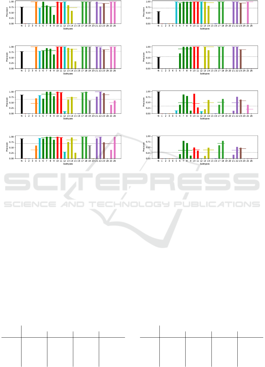
Figure 8: Evaluation of per-subtype test set classification. Lines spanning multiple bars of the same color mark supertype
classification performance for each class. Dashed line indicates an average score. The color code corresponds to that in Figure
6.
5.3.1 Average F
0.5
-scores
In Tables 1 and 2 we compare the F
0.5
-scores achieved
with our models. The similarity metric mse presents
the best average performance in both supertype and
subtype classification. The highest F
0.5
-score is
achieved with the color space L*a*b*. YIQ and RGB
perform just a little poorer due to a lower recall. Mod-
els trained with r perform better only in training set
classification because of the descriptor bias.
Our method of descriptor construction with dis-
placement provides an improved subtype prediction
F
0.5
-score by 0.15 on the training set and 0.08 on the
test set on mse models. In r-models this improve-
ment is lower: at around 0.06 and 0.05. For supertype
Table 1: F
0.5
-scores achieved during costume subtype clas-
sification.
color mse
d
mse r
b
r
space train test train test train test train test
RGB 0.85 0.61 0.65 0.54 0.67 0.34 0.57 0.29
YIQ 0.85 0.64 0.72 0.55 0.90 0.52 0.84 0.41
0IQ 0.76 0.49 0.63 0.44 0.83 0.31 0.87 0.25
L*a*b* 0.91 0.69 0.74 0.62 0.87 0.42 0.81 0.37
0a*b* 0.77 0.56 0.66 0.45 0.79 0.24 0.84 0.19
prediction these scores are only a little reduced with
0.09 and 0.12 in YIQ, and 0.1 and 0.05 in L*a*b*
color spaces for the mse-models. In r-models this
rise is comparable to subtype classification with 0.07
and 0.04 for both, YIQ and L*a*b* color models. It
is interesting to note that in the r-models, the F
0.5
-
score deteriorates slightly on the training set in color
spaces without luminosity data, presumably taking
away some of classifier bias.
5.3.2 Performance per Class
We now focus on the two color spaces with the
most promising classification performance – YIQ and
L*a*b*. Classification results of mse and r models
Table 2: F
0.5
-scores achieved during costume supertype
classification.
color mse
d
mse r
b
r
space train test train test train test train test
RGB 0.89 0.74 0.73 0.65 0.72 0.44 0.64 0.37
YIQ 0.90 0.74 0.81 0.62 0.91 0.59 0.84 0.48
0IQ 0.78 0.56 0.67 0.53 0.83 0.42 0.88 0.33
L*a*b* 0.92 0.77 0.82 0.72 0.88 0.47 0.81 0.43
0a*b* 0.78 0.59 0.72 0.59 0.79 0.33 0.83 0.26
Image-based Classification of Swiss Traditional Costumes using Contextual Features
419

are shown in Figure 8 for each subtype. It is apparent
that both, mse and r models have failed to learn some
of the subtypes. Nevertheless, the mse model was able
to distinguish more classes in both color spaces com-
pared to the r model. The mse model also presents a
more balanced performance in terms of precision and
recall.
Low classification precision of negative samples
in r models indicates that many positive samples have
been rejected during classification and assigned to the
rejection class. This is, again, explained by the clas-
sifier bias. Furthermore, this assumption is confirmed
by the high recall score of the rejection class, mean-
ing that most of true negative samples have been clas-
sified correctly and low precision is a result of erro-
neously rejected positive samples.
Note that supertype classification still holds a high
overall performance, even when some subtypes have
not been recognized. This means that samples in
those subtypes have been assigned to a sibling sub-
type, contributing to a better supertype classification
overall. It is worth noting, that only supertypes with
just one subtype have not been recognized. Poor
classification performance also correlates with low
amount of samples available for each class.
6 CONCLUSION
It is evident that the Swiss traditional costume dataset
is desperately small, but this is also the rationale for
this work. We use poselets, similar to (Chen et al.,
2012), to define reproducible features that cannot be
located visually. We also propose to compute descrip-
tors for features by iteratively merging sample im-
ages of these features, while allowing for displace-
ment during pair-wise comparisons. We demonstrate
that the F
0.5
-score of mse-models computed with dis-
placement increases by 0.07-0.12 on the test set, com-
pared to F
0.5
-score without displacement. This model
performs best in L*a*b* color space on both, subtype
and supertype costume classification.
REFERENCES
Cao, Z., Hidalgo, G., Simon, T., Wei, S.-E., and Sheikh,
Y. (2018). OpenPose: realtime multi-person 2D pose
estimation using Part Affinity Fields. In arXiv preprint
arXiv:1812.08008.
Cao, Z., Simon, T., Wei, S.-E., and Sheikh, Y. (2017). Real-
time multi-person 2d pose estimation using part affin-
ity fields. In CVPR.
Chen, H., Gallagher, A., and Girod, B. (2012). Describ-
ing clothing by semantic attributes. In Fitzgibbon, A.,
Lazebnik, S., Perona, P., Sato, Y., and Schmid, C., ed-
itors, Computer Vision – ECCV 2012, pages 609–623,
Berlin, Heidelberg. Springer Berlin Heidelberg.
Eichner, M., Marin-Jimenez, M., Zisserman, A., and Fer-
rari, V. (2012). 2d articulated human pose estimation
and retrieval in (almost) unconstrained still images.
International journal of computer vision, 99(2):190–
214.
Kalantidis, Y., Kennedy, L., and Li, L.-J. (2013). Getting
the look: clothing recognition and segmentation for
automatic product suggestions in everyday photos. In
Proceedings of the 3rd ACM conference on Interna-
tional conference on multimedia retrieval , pages 105–
112. ACM.
Liu, Z., Luo, P., Qiu, S., Wang, X., and Tang, X. (2016).
Deepfashion: Powering robust clothes recognition and
retrieval with rich annotations. In Proceedings of
the IEEE conference on computer vision and pattern
recognition, pages 1096–1104.
Lowe, D. G. (1999). Object recognition from local scale-
invariant features. In Computer vision, 1999. The pro-
ceedings of the seventh IEEE international conference
on, volume 2, pages 1150–1157. Ieee.
Varma, M. and Zisserman, A. (2005). A statistical approach
to texture classification from single images. Interna-
tional journal of computer vision, 62(1-2):61–81.
Wei, S.-E., Ramakrishna, V., Kanade, T., and Sheikh, Y.
(2016). Convolutional pose machines. In CVPR.
Yamaguchi, K., Kiapour, M. H., Ortiz, L. E., and Berg,
T. L. (2012). Parsing clothing in fashion photographs.
In Computer Vision and Pattern Recognition (CVPR),
2012 IEEE Conference on, pages 3570–3577. IEEE.
VISAPP 2020 - 15th International Conference on Computer Vision Theory and Applications
420