Corner Detection in Manifold-valued Images and in Vector Fields
Aleksei Shestov and Mikhail Kumskov
Faculty of Mechanics and Mathematics, Lomonosov Moscow State University, 1 Leninskiye Gory, Moscow, Russia
Keywords:
Corner Detection, Manifold-valued Images, Vector Fields, Vector Bundles.
Abstract:
This paper is devoted to the problem of corner detection in manifold-valued images and in vector fields on
manifolds. Our solution is a generalization of the Harris corner detector (C. Harris, 1988). As in the grayscale
case, our algorithm is based on an estimation of a self-similarity of a point neighborhood. We define the self-
similarity for the general cases and obtain approximations of it by an action of a bilinear form. This form can
be viewed as a generalization of the structure tensor (M. Kass, 1987). The generalized structure tensor is then
used as usual in the corner detection procedure. Finally, we describe future experiments: the algorithm will be
tested on a task of chemical compounds classification.
1 INTRODUCTION
In many applications and practical cases we process
non-Euclidean data. Images with values on the cir-
cle (periodic data) are met in applications involv-
ing the phase of Fourier transform (J. Bioucas-Dias,
2008; C.-A. Deledalle, 2011), interferometric syn-
thetic aperture radar(R. Bergmann, 2014), or hue-
component of an image. Spherical data appear when
dealing with 3d directional information (R. Kim-
mel, 2002; L. A. Vese, 2002) or with color images
in chromaticity-brightness color space (T. F. Chan,
2001). SO(3)-valued data are processed in elec-
tron backscattered tomography (F. Bachmann, 2011;
R. Bergmann, 2016). Images with values in the sym-
metric positive-definite matrices space are met in DT-
MRI imaging (C. ChefdHotel, 2004; P. T. Fletcher,
2004) or in processing covariance matrices associated
to image pixels (O. Tuzel, 2008).
Manipulating tangent vector fields is a fundamen-
tal operation in areas such as dynamic systems, finite
elements and geometry processing (Azencot et al.,
2013). Also, numerous applications in computer
graphics require to manipulate tangent vector fields
on surfaces, for example, texture synthesis, non-
photorealistic rendering, computer-generated movies,
animation (Goes et al., 2015).
One approach to the manifold data processing is
a generalization of grayscale image processing meth-
ods. Harris corner detector is a widely used method of
keypoints detection in grayscale images. It has appli-
cations in image alignment, stitching, registration, 2d
mosaics creation, 3d scene modeling and reconstruc-
tion, motion detection, object recognition, etc. The
goal of the algorithm is to find points which neighbor-
hoods are not self-similar in any direction, opposed to
edges, which are self-similar in one direction, and to
flat surfaces, which are self-similar in any direction.
Self-similarity is assessed by the sum of squared dif-
ferences between a region and a shifted region. This
sum is approximated by an action of a bilinear form,
called the structure tensor (M. Kass, 1987). A cor-
ner response is calculated from the eigenvalues of the
structure tensor, and corners are found as local maxi-
mums of the corner response.
Our goal is to develop a generalization of the Har-
ris corner detector for the general settings of a). an
image being a map between manifolds and b). an
image being a vector field on a manifold. The main
question of the generalization is deriving the structure
tensor. In order to derive it, we start from definitions
of the self-similarity of a point neighborhood. These
definitions are similar to the grayscale case, but have
some modifications: in the manifold case we substi-
tute the distances on the manifold for the differences,
in the vector field case we use the parallel transport.
Then we derive approximations of the self-similarity
by the action of the bilinear form, which matrix con-
sists of the image derivatives and the image metric.
This bilinear form can be viewed as a generalization
of the structure tensor. The generalized structure ten-
sor is used as usual in the corner detection procedure.
Shestov, A. and Kumskov, M.
Corner Detection in Manifold-valued Images and in Vector Fields.
DOI: 10.5220/0009102304050411
In Proceedings of the 15th International Joint Conference on Computer Vision, Imaging and Computer Graphics Theory and Applications (VISIGRAPP 2020) - Volume 4: VISAPP, pages
405-411
ISBN: 978-989-758-402-2; ISSN: 2184-4321
Copyright
c
 2022 by SCITEPRESS – Science and Technology Publications, Lda. All rights reserved
405

Contributions:
1. We are the first to provide the Harris corner detec-
tor generalization for the cases of an image being
a map between manifolds and an image being a
vector field on a manifold.
2. We are the first to provide an interest point detec-
tor for the case of an image being a vector field on
a manifold.
2 THE HARRIS CORNER
DETECTOR OVERVIEW
Let’s start from a description of the Harris corner de-
tector for the grayscale case. The setting of the prob-
lem is the following. Let f : R
n
→ R be a grayscale
image. We want to find points which neighborhoods
have a low self-similarity. The self-similarity is as-
sessed by the sum of squared differences between a
neighborhood and a shifted neighborhood:
selfsim(ε∆x) =
Z
U(x
0
)
w(x)

f (x + ε∆x) − f (x)

2
dx,
where ∆x is a direction in which we estimate the self-
semilarity, k∆xk = 1, U(x
0
) is a neighborhood of in-
terest, w(x) is a weight function, the Gaussian func-
tion is usually chosen as w(x).
Earlier corner detectors(Moravec, 1980) tried to
calculate this quantity directly. The direct calculation
has such drawback that a number of directions ∆x,
in which we can calculate selfsim, is limited. In the
Harris corner detector this problem is solved by using
an approximation of selfsim by the Taylor expansion.
The expressions are the following:
f (x + ε∆x) − f (x) = ε
∑
i
∂ f
∂x
i
(x)∆x
i
+ o(ε);

f (x + ε∆x) − f (x)

2
= ε
2
∑
i, j
∂ f
∂x
i
∂ f
∂x
j
∆x
i
∆x
j
+
+ o(ε
2
) = ε∆x

d f
T
x
d f
x

ε∆x
T
+ o(∆ f
2
)
selfsim(ε∆x) =
Z
U(x
0
)
w(x)

f (x + ε∆x)−
− f (x)

2
dx = ε∆x

Z
U(x
0
)
w(x)

d f
T
x
d f
x

dx

ε∆x
T
+
+ o(selfsim);
So selfsim(ε∆x) for small values of ε is approx-
imated by the action of the bilinear form S =
R
U(x
0
)
w(x)

d f
T
x
d f
x

dx. This bilinear form is called
the structure tensor.
The whole corner detection algorithm is the fol-
lowing:
1. Calculate the structure tensor for ever pixel of an
image
2. Calculate a corner response. In the article(Tomasi
and Kanade, 1991) it’s suggested to use the
direction-wise minimum of the self-similarity,
which is estimated from the eigenvalues of S.
In(C. Harris, 1988) another response expression is
used: R = detS − k(trS)
2
. A usage of this expres-
sion is computationally cheaper than a direct esti-
mation of the eigenvalues of S, because it doesn’t
involve the square root calculation.
3. Corners are found as local maximums of the cho-
sen response, which have a high response value.
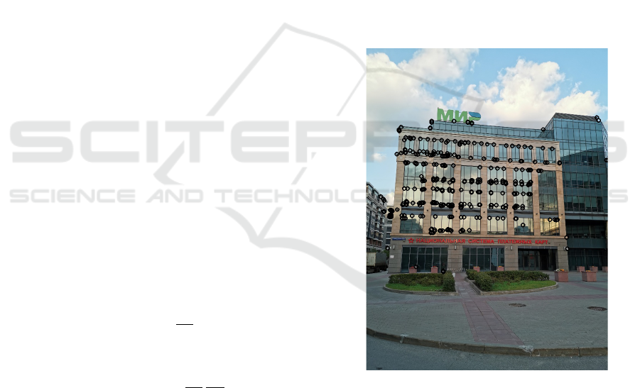
An example of the Harris corner detection result is
presented in Fig. 1.
Figure 1: An image with found corners (denoted by black
circles) on it.
A generalization of the Harris corner detector for
color images was proposed in the articles(Montesinos
et al., 1998; Montesinos et al., 2000). In these articles
a norm of difference is used in selfsim:
selfsim(ε∆x) =
Z
U(x
0
)
w(x)k

f (x + ε∆x)− f (x)

k
2
dx.
This leads to the same expression for the matrix of the
structure tensor, except now d f
x
is a 3 × n matrix.
VISAPP 2020 - 15th International Conference on Computer Vision Theory and Applications
406

How can this algorithm be generalized to the more
general data types? We can see that the real problem
is the step 1 of the algorithm, the structure tensor cal-
culation. So the main question is how to define the
structure tensor. We will follow the next scheme:
1. We will define the self-similarity for the consid-
ered case. We can’t straightforwardly use the self-
similarity of the grayscale case, because some op-
erations of it are not defined in the general case.
So some modifications should be done to the self-
similarity definition.
2. We will approximate the defined self-similarity
for the small shifts by an action of a bilinear form,
in order to be able to assess the self-similarity in
every direction. This bilinear form will be used as
the structure tensor in the corner detection algo-
rithm.
3 THE MANIFOLD CASE
Let us present our solution for the manifold case.
In this case an image is a map between manifolds:
f (x) : X → Y , where X and Y are Riemannian mani-
folds, dim(X) = n, dim(Y ) = m. Here and further all
manifolds and functions are considered to be smooth.
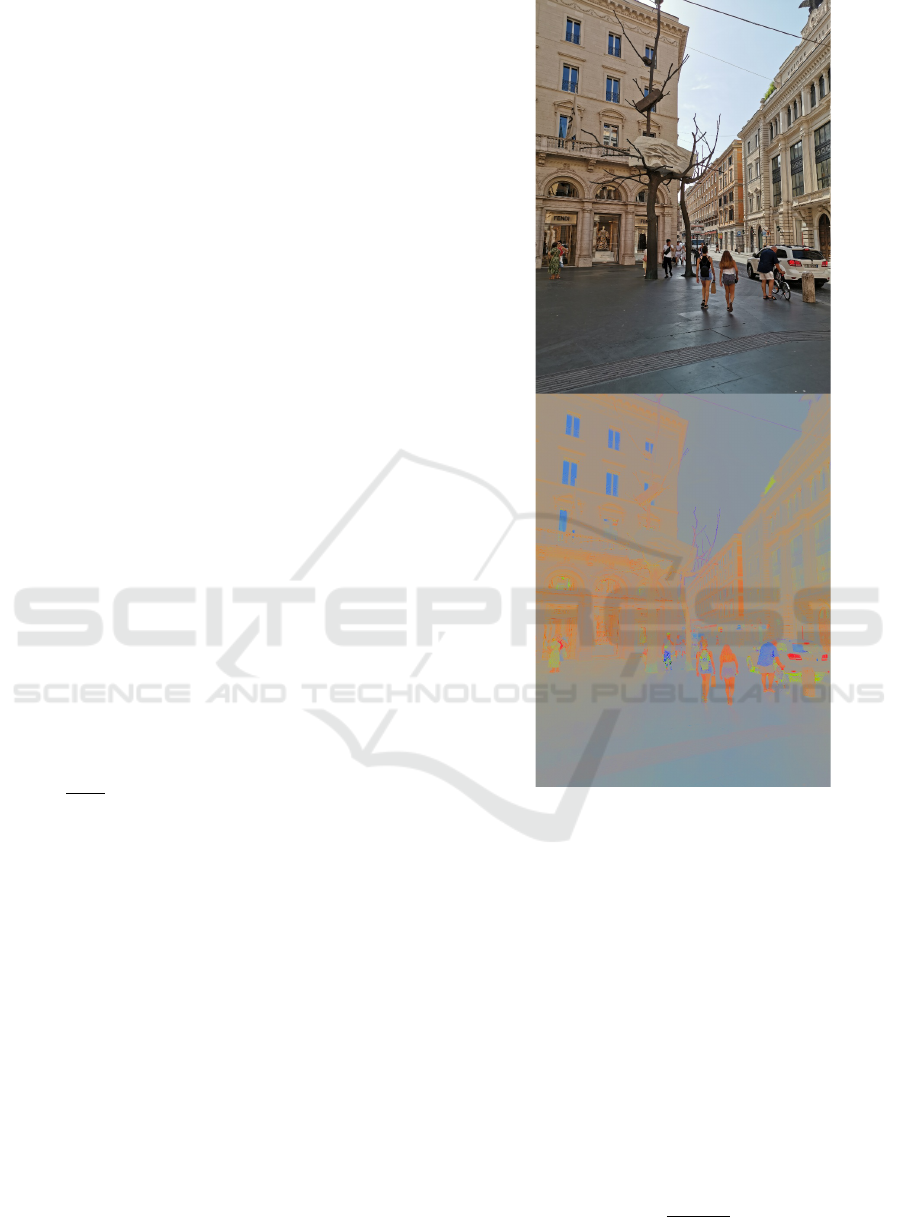
A practical situation, corresponding to this general
setting, could be, the following: f is a chromaticity
component of an image in the chromaticity-brightness
color space(T. F. Chan, 2001). In the chromaticity-
brightness model an RGB pixel value I(x) is decom-
posed into 2 components — the brightness compo-
nent u(x) = kI(x)k, and the chromaticity component
f (x) =
I(x)
kI(x)k
(see Fig. 2). The chromaticity compo-
nent f (x) ”lives” on a unit sphere S
2
. So for this case
X = A ⊂ R
2
, Y = S
2
.
At first, we should define the self-similarity for
the considered case. As now f (x) and f (x + ε∆x) are
points on the manifold Y , we can’t take the difference
of them, because the difference is not defined in gen-
eral. Instead we propose to take a length of the short-
est path, connecting them on Y , as the distance. So
self-similarity is defined in the following way (here
x + ε∆x is a coordinate expression):
selfsim(ε∆x) =
Z
U(x
0
)
w(x)dist

f (x + ε∆x), f (x)

2
dx,
where k∆xk = 1. Then, as in the grayscale case, we
will approximate the self-similarity for small shifts by
the action of a bilinear form. This bilinear form can
be viewed as a generalization of the structure tensor
for the manifold case. The precise propositions are
given in the following theorem. Before it we should
state a few definitions.
Figure 2: An image in the RGB space and its chromaticity
component under it.
Definition 1. Let M be a smooth manifold, dim(M) =
n, x ∈ M. Pick a coordinate chart φ : U → R
n
, x ∈ U,
U ⊂ M. Let there be two curves γ
1
, γ
2
: (−1, 1) → M,
γ
1
(0) = γ
2
(0) = x. γ
1
and γ
2
are equivalent at x if and
only if the derivatives of φ◦ γ
1
and φ ◦γ
2
at 0 coincide.
Equivalence classes, defined in that way, are tangent
vectors of M at x. Then the tangent space of M at x,
denoted by T
x
M, is a set of all tangent vectors of M at
x. T
x
M forms a linear space of dim(T
x
M) = n.
Definition 2. Let M be a smooth manifold, dim(M) =
n, x ∈ M. A metric tensor of M at x is a symmetric
positive-definite bilinear form g
M
x
, which acts on vec-
tors of the tangent space T
x
M. The length of a vector
v ∈ T
x
M is defined as
p
g
M
x
(v, v).
Corner Detection in Manifold-valued Images and in Vector Fields
407

Theorem 1.
selfsim(ε∆x) =
= ε∆x

Z
U(x
0
)
w(x)

d f
T
x
G
Y
f (x)
d f
x

dx

ε∆x
T
+
+ o(selfsim),
where d f
x
is an m ×n matrix of the differential of f at
the point x,
G
Y
f (x)
is an m×m matrix of the metric of Y at the point
f (x).
The matrix
R
U(x
0
)
w(x)

d f
T
x
G
Y
f (x)
d f
x

dx is the mani-
fold structure tensor.
Proof. At first, let’s approximate the distance be-
tween f (x) and f (x+ε∆x) by their per-coordinate dif-
ference. Let γ(t) be the shortest curve in the natural
parametrization connecting them: γ(0) = f (x), γ(s) =
f (x + ε∆x), s = dist( f (x), f (x + ε∆x)). Then by the
Taylor expansion of γ:
f (x + ε∆x) − f (x) =
˙
γ(0)s + o(s).
Here f (x + ε∆x) − f (x) = ∆ f is a coordinate expres-
sion,
˙
γ(0) is a vector in the coordinates of T
f (x)
Y ,
˙
γ(0) has a unit length. From this it also follows that
∆ f = O(s). Then substitute this expression for the
squared length of
˙
γ(0)s:
s
2
g
Y
y
(
˙
γ(0),
˙
γ(0)) = g
Y
y
(∆ f , ∆ f ) + o(s
2
),
where g
Y
y
is a metric tensor of Y at the point y = f (x).
dist( f (x), f (x + ε∆x))
2
= g
Y
y
(∆ f , ∆ f ) + o(dist
2
).
Let’s approximate ∆ f by the Taylor expansion: ∆ f =
d f
x
(ε∆x) + o(ε). Then
g
Y
y
(∆ f , ∆ f ) = g
Y
y
(d f
x
(ε∆x), d f
x
(ε∆x)) + o(ε
2
).
From the Taylor expansions: ε = O(∆ f ) = O(dist).
Then
dist( f (x), f (x + ε∆x))
2
=
= g
Y
y
(d f
x
(ε∆x), d f
x
(ε∆x)) + o(dist
2
) =
= ε∆x


d f
T
x
G
Y
f (x)
d f
x

dx

ε∆x
T
+ o(dist
2
).
Then
selfsim(ε∆x) =
=
Z
U(x
0
)
w(x)dist

f (x + ε∆x), f (x)

2
dx =
= ε∆x

Z
U(x
0
)
w(x)

d f
T
x
G
Y
f (x)
d f
x

dx

ε∆x
T
+
+ o(selfsim)
So we approximated the self-similarity
by the action of the bilinear form S =
R
U(x
0
)
w(x)

d f
T
x
G
Y
f (x)
d f
x

dx. This bilinear form
will be called the manifold structure tensor. It is
then used as usual in the corner detection procedure:
we calculate the corner response as the minimal
eigenvalue of S, or calculate R = det S − k(tr S)
2
.
Corners are found as local maximums of the chosen
response, which have high response values.
4 THE VECTOR FIELD CASE
Let us proceed to the case of image being a vector
field on a manifold. Before going into more detailed
discussion we need to state a few definitions.
At first, let us discuss the notion of the vector bun-
dle. Informally, the idea is the following: to every
point x of the manifold X we attach a vector space
V (x) in such a way that these vector spaces fit together
to form another manifold E, which is then called a
vector bundle over X . I.e. vector bundles are spaces,
where vector fields on a manifold ”live”. The formal
definition is the following:
Definition 3. A vector bundle (E, X, π) consists of
manifolds X (base space), E (total space) and a con-
tinuous surjection π : E → X (bundle projection). For
every x ∈ X π
−1
(x) (called a fiber) has the structure
of a finite-dimensional vector space. The following
condition is satisfied: for every point x ∈ X, there is
an open neighborhood U ⊂ X of x, and a homeomor-
phism
φ : U × R
m
→ π
−1
(U)
such that for all x ∈ U,
1. (π ◦ φ)(x, v) = x for all v ∈ R
m
,
2. the map v 7→ φ(x, v) is a linear isomorphism be-
tween the vector spaces R
m
and π
−1
(x).
Elements of a vector bundle are called sections of
a vector bundle. A section of a vector bundle can be
simply viewed as a vector field on a manifold. The
tangent bundle is also a vector bundle.
Proceed to the notion of the covariant derivative.
The covariant derivative is a rule of calculating a
derivative of sections of vector bundles. The formal
definition is the following:
Definition 4. A covariant derivative ∇ at a point x
in a smooth manifold X assigns a section (∇
v
u)
x
to a
pair of a tangent vector v at x and a vector field u de-
fined in a neighborhood of x, such that the following
properties hold:
VISAPP 2020 - 15th International Conference on Computer Vision Theory and Applications
408

1. ∇
v
u is linear in v:
∇
gv
1
+ f v
2
u = g∇
v
1
u + f ∇
v
2
u;
2. ∇
v
u is additive in u:
∇
v
u
1
+ u
2
= ∇
v
u
1
+ ∇
v
u
2
;
3. ∇
v
u obeys the product rule:
∇
v
f u = f (x)∇
v
u + u(x)∇
v
f
Now let us review the notion of the parallel trans-
port. Informally speaking, the parallel transport is a
way of transporting vectors from different fibers of
a vector bundle along smooth curves in a manifold,
so that they stay parallel with respect to the covariant
derivative. The formal definition is the following:
Definition 5. Let (E, X , π) be a vector bundle over X ,
let e ∈ E
x
at x = γ(0) ∈ X. The parallel transport of e
along γ is the extension of e to the unique section u of
E along γ such that:
1. ∇
˙
γ
u = 0;
2. u
γ(0)
= e.
Then return to our problem. Let there be a man-
ifold X , dim(X) = n, a vector bundle (E, X , π) over
X, dim(E) = m, and let f be a section of this vector
bundle ( f is a vector field on X). A particular case,
corresponding to this general setting, could be, for
example, the following: X is a 2d surface and f is
a tangent vector field on X.
At first, we should define the self-similarity for the
considered case. In this case f (x) and f (x + ε∆x) are
elements of different fibers, so we can’t take a dif-
ference of them. In order to manipulate them, these
vectors should be moved by the parallel transport to
the same fiber. So the self-similarity is defined in the
following way (here x + ε∆x is a coordinate expres-
sion):
selfsim(ε∆x) =
=
Z
U(x
0
)
w(x)k f (x + ε∆x) − Γ
x+ε∆x
x
( f (x))k
2
dx,
where k∆xk = 1, Γ
x+ε∆x
x
denotes the parallel transport
from x to x + ε∆x along the shortest curve, connect-
ing x and x + ε∆x. We assume that all operations take
place in the normal neighborhood of x, that is a neigh-
borhood, in which there is only one shortest curve,
connecting each pair of points. Then, as in all previ-
ous cases, we will approximate the self-similarity for
small shifts by the action of a bilinear form, which can
be viewed as a generalization of the structure tensor
to the vector field case. The formal expressions are
given by the following theorem:
Theorem 2.
selfsim(ε∆x) =
= ε∆x

Z
U(x
0
)
w(x)

∇ f
T
x
G
E
x
∇ f
x

dx

ε∆x
T
+
+ o(selfsim),
where ∇ f
x
is an m × n matrix of the covariant dif-
ferential of f at the point x, i.e. a matrix consist-
ing of covariant derivatives of f by the basis vectors:
∇ f
x
(i, j) = (∇
e
j
f )(i)
G
E
x
is an m × m matrix of the metric of E at the point
x.
The matrix
R
U(x
0
)
w(x)

∇ f
T
x
G
E
x
∇ f
x

dx is the vector
field structure tensor.
Proof. At first let’s review the difference of the vec-
tors:
f (x + ε∆x) − Γ
x+ε∆x
x
( f (x)) =
=
ε( f (x + ε∆x) − Γ
x+ε∆x
x
( f (x)))
ε
=
= (by one of the properties) ε(∇
∆x
f )
x+ε∆x
+ o(ε).
Let x
1
= x + ε∆x. Then substitute this to the squared
norm:
kε(∇
∆x
f )
x
1
+ o(ε)k
2
=
= g
E
x
1
(ε(∇
∆x
f )
x
1
, ε(∇
∆x
f )
x
1
) + o(ε
2
) =
= (g
E
x
+ o(ε))(ε(∇
∆x
f )
x
+ o(ε), ε(∇
∆x
f )
x
+ o(ε))+
+ o(ε
2
) = ε∆x

∇ f
T
x
G
E
x
∇ f
x

ε∆x
T
+ o(ε
2
).
From the Taylor expansion of f o(ε
2
) = o(∆ f
2
).
Combine this with the self-similarity definition and
obtain:
selfsim(ε∆x) =
=
Z
U(x
0
)
w(x)k f (x + ε∆x) − Γ
x+ε∆x
x
( f (x))k
2
dx =
= ε∆x

Z
U(x
0
)
w(x)

∇ f
T
x
G
E
x
∇ f
x

dx

ε∆x
T
+
+ o(selfsim).
With this theorem we approximated the self-
similarity by the action of the bilinear form S =
R
U(x
0
)
w(x)

∇ f
T
x
G
E
x
∇ f
x

dx. This bilinear form will
be called the vector field structure tensor. It is then
used as usual in the corner detection procedure: we
calculate the corner response as the minimal eigen-
value of S, or calculate R = detS − k(tr S)
2
. Corners
are found as local maximums of the chosen response,
which have high response values.
Corner Detection in Manifold-valued Images and in Vector Fields
409

5 THE EXPERIMENTS
Regarding the experiments our work now is a work in
progress. Here we will describe the future experimen-
tal setup and the algorithm implementation. These ex-
periments were not conducted yet.
5.1 Experimental Setup
We will apply our blob detection framework to
a chemical compounds classification problem, also
called the QSAR problem (Baskin and Varnek, 2009).
The task is to predict the activity of the compounds
using their structure. Each compound is represented
by a triangulated molecular surface (Connolly, 1983)
and several physico-chemical and geometrical proper-
ties on the surface. We use the following properties:
the electrostatic and the steric potentials, the Gaus-
sian and the mean curvatures, the directions of elec-
trostatic and steric forces, the gradients of the scalar
properties. These properties are calculated in each
triangulation vertex. So an input data element can
be modeled as a 2-dimensional manifold X with a
combined function ( f
1
, f
2
, f
3
): f
1
(x) : X → R
4
(the
scalar properties), f
2
(x) : X → S
2
× S
2
(the direc-
tional properties), f
3
is a section of the vector bundle
T X ⊗ T X ⊗ T X ⊗ T X (the gradient properties). An
example of input data is presented in Fig. 3.
Figure 3: A molecular surface of a glycoside compound
with the Gaussian curvature on it, denoted by color. Green
is for low values, red is for high values.
5.2 Implementation
We use the manifold and vector field corner detectors
for the construction of descriptor vectors. The proce-
dure is the following:
1. Detect corners by our method on each compound
surface;
2. Form pairs of corners on each surface;
3. Transform the corners pairs into vectors of the
same length by using the bag of words approach
(Csurka et al., 2004).
The implementation of the procedure of the corner de-
tection is the following:
1. Calculate the differentials of each component
of f
1
and f
2
by the approach following(Barth,
1993). The differentials of f
2
are calculated for
each coordinate φ and θ of the spherical coor-
dinate system. The overall differentials d f
1
and
d f
2
are obtained by stacking per-component dif-
ferentials: d f
1
= (d f
11
, d f
12
, d f
13
, d f
14
), d f
2
=
(d f
21φ
, d f
21θ
, d f
22φ
, d f
22θ
). The procedure of the
differentials d f
ik
calculation is the following:
• Find the directional derivatives ∂
z
j
f
ik
by the fi-
nite differences approximation, where z
j
are the
directions from v to its neighbour vertices.
• Find the differential d f
i
= (d f
ik
) by solving the
overdetermined linear system d f (Z) = ∂
z
j
f
ik
,
Z is a matrix which columns are vectors z
j
.
2. Calculate the covariant differentials ∇ f
3k
of
each component of f
3
by the approach fol-
lowing(Liu et al., 2016). The overall co-
variant differential ∇ f
3
is obtained by stack-
ing per-component covariant differentials ∇ f
3
=
(∇ f
31
, ∇ f
32
, ∇ f
33
, ∇ f
34
)
3. Calculate matrices under the integral of the struc-
ture tensor definition
• Calculate S
01
= d f
T
1
G
R
4
f
1
(x)
d f
1
(see the Theo-
rem 1) for f
1
. For the f
1
case the matrix G
R
4
f
1
(x)
is simply a unit matrix.
• Calculate S
02
= d f
T
2
G
S
2
×S
2
f
2
(x)
d f
2
(see the Theo-
rem 1) for f
2
. For the f
2
case the matrix G
S
2
×S
2
f
2
(x)
is found by the standard formulas for the spher-
ical coordinate system.
• Calculate S
03
= ∇ f
T
3
G
T X
4
x
∇ f
3
(see the Theo-
rem 2) for f 3. For the f
3
case the matrix G
T X
4
x
is simply a unit matrix, because we chose an
orthonormal coordinate system at each vertex.
• Calculate S
0
= S
01
+ S
02
+ S
03
.
4. For each vertex calculate the structure tensor
S(x
0
) =
R
U(x
0
)
w(x)S
0
dx with different values of
w(x). We choose the Gaussian function with dif-
ferent values of σ as w(x).
5. Detect corners as local maximums of the corner
response R = detS − k(tr S)
2
for each value of σ
of w(x).
6 CONCLUSION
We propose the framework for the corner detection
in manifold-valued images and in vector fields over
VISAPP 2020 - 15th International Conference on Computer Vision Theory and Applications
410

manifolds. This framework is based on the approxi-
mation of the self-similarity by the action of the struc-
ture tensor. Both the self-similarity and the structure
tensor are derived in our work for the general cases.
Our approach gives new methods for the uncovered
problems. The future experiments and the implemen-
tation are described. The next direction for the re-
search is the described experiment.
REFERENCES
Azencot, O., BenChen, M., Chazal, F., and Ovsjanikov, M.
(2013). An operator approach to tangent vector field
processing. Computer Graphics Forum, 32.
Barth, T. J. (1993). A 3-d least-squares upwind euler solver
for unstructured meshes. In Napolitano, M. and Sa-
betta, F., editors, Thirteenth International Conference
on Numerical Methods in Fluid Dynamics, pages 240–
244, Berlin, Heidelberg. Springer Berlin Heidelberg.
Baskin, I. and Varnek, A. (2009). ChemInform Abstract:
Fragment Descriptors in SAR/QSAR/QSPR Studies,
Molecular Similarity Analysis and in Virtual Screen-
ing, volume 40, pages 1–43.
C.-A. Deledalle, L. Denis, F. T. (2011). Nl-insar: Nonlo-
cal interferogram estimation. IEEE Transactions on
Geoscience Remote Sensing, (49):1441–1452.
C. ChefdHotel, D. Tschumperle, R. D. O. F. (2004).
Regularizing flows for constrained matrix-valued im-
ages. Journal of Mathematical Imaging and Vision,
(20):147–162.
C. Harris, M. S. (1988). A combined corner and edge de-
tector. In Alvey Vision Conference.
Connolly, M. L. (1983). Analytical molecular surface
calculation. Journal of Applied Crystallography,
16(5):548–558.
Csurka, G., Dance, C., Fan, L., Willamowski, J., and Bray,
C. (2004). Visual categorization with bags of key-
points. Work Stat Learn Comput Vision, ECCV, Vol.
1.
F. Bachmann, R. Hielscher, H. S. (2011). Grain detection
from 2d and 3d ebsd data - specification of the mtex
algorithm. Ultramicroscopy, (111):1720–1733.
Goes, F., Desbrun, M., and Tong, Y. (2015). Vector field
processing on triangle meshes.
J. Bioucas-Dias, V. Katkovnik, J. A. K. E. (2008). Absolute
phase estimation: adaptive local denoising and global
unwrapping. Applied Optics, (47):5358–5369.
L. A. Vese, S. J. O. (2002). Numerical methods for p-
harmonic flows and applications to image process-
ing. SIAM Journal on Numerical Analysis, (40):2085–
2104.
Liu, B., Tong, Y., Goes, F., and Desbrun, M. (2016).
Discrete connection and covariant derivative for vec-
tor field analysis and design. ACM Transactions on
Graphics, 35.
M. Kass, A. W. (1987). Analyzing oriented patterns.
Computer Vision, Graphics, and Image Processing,
(37):362–385.
Montesinos, P., Gouet, V., and Deriche, R. (1998). Dif-
ferential invariants for color images. In Proceed-
ings of the 14th International Conference on Pattern
Recognition-Volume 1 - Volume 1, ICPR ’98, Wash-
ington, DC, USA. IEEE Computer Society.
Montesinos, P., Gouet, V., Deriche, R., and Pel, D. (2000).
Matching color uncalibrated images using differential
invariants. Image Vision Comput., 18:659–671.
Moravec, H. P. (1980). Obstacle Avoidance and Naviga-
tion in the Real World by a Seeing Robot Rover. PhD
thesis, Stanford, CA, USA. AAI8024717.
O. Tuzel, F. Porikli, P. M. (2008). Learning on lie groups
for invariant detection and tracking. In CVPR 2008,
pages 1–8. IEEE.
P. T. Fletcher, S. J. (2004). Principal geodesic analysis on
symmetric spaces: Statistics of diffusion tensors. In
Computer Vision and Mathematical Methods in Med-
ical and Biomedical Image Analysis, volume 3117,
pages 87–98. Springer.
R. Bergmann, F. Laus, G. S. A. W. (2014). Second order
differences of cyclic data and applications in varia-
tional denoising. SIAM Journal on Imaging Sciences,
(7):2916–2953.
R. Bergmann, R. H. Chan, R. H. J. P. G. S. (2016). Restora-
tion of manifold-valued images by half-quadratic min-
imization. Inverse Problems in Imaging, (10):281–
304.
R. Kimmel, N. S. (2002). Orientation diffusion or how to
comb a porcupine. Journal of Visual Communication
and Image Representation, (13):238–248.
T. F. Chan, S. Kang, J. S. (2001). Total variation denoising
and enhancement of color images based on the cb and
hsv color models. Journal of Visual Communication
and Image Representation, (12):422–435.
Tomasi, C. and Kanade, T. (1991). Detection and tracking
of point features. Technical report, International Jour-
nal of Computer Vision.
Corner Detection in Manifold-valued Images and in Vector Fields
411