Variable Selection based on a Two-stage Projection Pursuit Algorithm
Shu Jiang
1
and Yijun Xie
2
1
Division of Public Health Sciences, Department of Surgery, Washington University in St. Louis, St. Louis, U.S.A.
2
Department of Statistics and Actuarial Science, University of Waterloo, Waterloo, Canada
Keywords:
Two-stage Projection Pursuit, Variable Selection, Optimization.
Abstract:
Dimension reduction methods have gained popularity in modern era due to exponential growth in data collec-
tion. Extracting key information and learning from all available data is a crucial step. Principal component
analysis (PCA) is a popular dimension reduction technique due to its simplicity and flexibility. We stress that
PCA is solely based on maximizing the proportion of total variance of the explanatory variables and do not
directly impact the outcome of interest. Variable selection under such unsupervised setting may thus be inef-
ficient. In this note, we propose a novel two-stage projection pursuit based algorithm which simultaneously
consider the loss in the outcome variable when doing variable selection. We believe that when one is keen in
variable selection in relation to the outcome of interest, the proposed method may be more efficient compared
to existing methods.
1 INTRODUCTION
Tremendous amounts of data are being collected in
the hopes of finding significant factors that may be
associated with, for example, disease progression in
clinical studies. With the exponential growth in data
collection, a natural question is how to select a smaller
subset of meaningful variables from the larger pool.
A naturally adopted method in overcoming such bur-
den is by dimensional reduction techniques. Principal
component analysis (PCA) has been arguably most
commonly adopted technique for such purpose. The
mathematical properties as well as highly optimized
algorithms for eigen-decomposition make PCA a very
appealing and prevalent technique for dimension re-
duction. More precise descriptions on relevant uses
of PCA can be found in Krzanowski (1987), King
and Jackson (1999), Cadima and Jolliffe (2001), and
Cadima et al. (2004).
We should note that, however, the fundamental
purpose of PCA decomposition is to maximize the
proportion of total variance of the explanatory vari-
ables explained by the principal components, and
therefore minimize the variance of residuals. Such
unsupervised approach focusing only on the vari-
ance decomposition of explanatory variables may
well mimic the structure of the variables, but does
not impact the relationship between the explanatory
variables and the outcome/response under a regres-
sion setting. Therefore, such unsupervised method
may not be the optimal approach if one’s goal lies in
dimensional reduction in relation to the outcome of
interest.
To overcome such burden, various efforts have
been made in developing projection pursuit based
methods for selecting the best set of variables. Monta-
nari and Lizzani (2001) discussed a projection pursuit
algorithm to identify multivariate variables for classi-
fication. Enshaei and Faith (2015) developed an al-
gorithm based on perceptron learning and attraction-
repulsion algorithms to find the variable that best sep-
arates the data. More relevantly, Hwang et al. (1994)
discussed projection pursuit learning algorithm for
regression-based problems.
One of the drawbacks of traditional projection
pursuit algorithm is that it requires considerable
amount of computing power. Such limitation pre-
vented previous efforts in implementing projection
pursuit in higher dimensional space. The computa-
tional burden has gotten worse in recent years due to
exponential increase in the number of variables being
collected in the dataset. Therefore we are motivated
to introduce a novel dimensional reduction technique,
the two-stage projection pursuit method, for variable
selection in high dimensional variable space. We
believe that the proposed two-stage procedure could
lead to the most efficient selection of the set of vari-
ables that exert relatively large effects on the outcome
188
Jiang, S. and Xie, Y.
Variable Selection based on a Two-stage Projection Pursuit Algorithm.
DOI: 10.5220/0009098901880193
In Proceedings of the 13th International Joint Conference on Biomedical Engineering Systems and Technologies (BIOSTEC 2020) - Volume 3: BIOINFORMATICS, pages 188-193
ISBN: 978-989-758-398-8; ISSN: 2184-4305
Copyright
c
 2022 by SCITEPRESS – Science and Technology Publications, Lda. All rights reserved

of interest without much computational burden.
This paper is organized as follows. We first re-
view the principal component analysis (PCA) and its
feature selection techniques in Section 2.1. We then
introduce a new dimension reduction framework for
high dimensional data based on a two-stage projec-
tion pursuit algorithm in Section 2.2. A detailed out-
line of our purposed algorithm is included in Sec-
tion 2.2.2. In Section 3 we conduct a small scale
simulation study to compare the performance of our
proposed algorithm with existing methods including
PCA. We present a data example in Section 4 and end
with a discussion in Section 5.
2 DIMENSION REDUCTION
2.1 Principal Component Analysis
Let X = [X
1
,··· , X
d
]
0
be a d-dimensional random vec-
tor with zero mean. We let v
m
= [v
m1
,··· , v
md
]
0
be a
vector of length d where the norm is defined as the
L
2
norm, i.e. ||v
m
|| = v
0
m
v
m
=
q
∑
d
j=1
v
2
m j
= 1. We
further let W
m
denote the inner product of v
m
and X ,
which is often referred to as the projection score of X
onto v
m
in the literature. Specifically,
W
m
= hv
m
,Xi =
d
∑
j=1
v
m j
X
j
. (1)
The first principal component W
1
can thus be defined
as
W
1
= hv
1
,Xi,
where
v
1
= argmax
v
m
∈R
d
,||v
m
||=1
Var(W
m
)
is the unit length vector in an R
d
space that maximizes
the variance of the projection scores. We can see from
above that the first principal component tries to find
a unit length vector in the d-dimensional Euclidean
space such that the projection score of a higher di-
mensional random vector onto this unit length vec-
tor has the maximum variance among all projection
scores. Such procedure will decompose the random
vector X into two parts: the projection that is in the
same direction as v
1
, and residuals that are orthogonal
to v
1
. Each subsequent v
k
is defined as the direction
that will maximize the variance of the residuals after
the (k − 1)
th
projection, i.e.
v
k
= argmax
v
m
∈R
d
,||v
m
||=1,
hv
m
,v
q
i=0 for q<k
Var(W
m
).
The k
th
principal component W
k
can then be writ-
ten as
W
k
= hv
k
,Xi.
The estimation of the components v
1
,...,v
k
involves
the covariance matrix Σ of X which is assumed to be
full rank. Specifically for v
1
, we would need to max-
imize v
0
1
Σv
1
subject to v
0
1
v
1
= 1 and one possible ap-
proach is to use Lagrange multipliers
v
0
1
Σv
1
+ λ(v
0
1
v
1
− 1), (2)
where λ is a constant. By differentiating (2) with re-
spect to v
1
we would get
(Σ − λI)v
1
= 0, (3)
where I is a d × d identity matrix. We can see from
(3) that λ is an eigenvalue of Σ and v
1
is the corre-
sponding eigenvector where
v
0
1
Σv
1
= v
0
1
λv
1
= λv
0
1
v
1
= λ.
Hence, the maximum of v
0
1
Σv
1
is achieved when λ =
λ
1
, the largest eigenvalue of Σ with v
1
the eigenvec-
tor corresponding to λ
1
. Similarly, one can show that
v
k
is the eigenvector corresponding to the k
th
largest
eigenvalue λ
k
. More details can be found in Jolliffe
(2011).
2.2 Projection Pursuit Algorithm
2.2.1 Methods and Notations
It is clear that PCA is targeted at maximizing the vari-
ance of the projection scores for some high dimen-
sional vector X. However, we stress that such unsu-
pervised approach may not always the optimal choice
when the goal for variable selection is associated with
the outcome of interest. We are thus motivated to in-
troduce an alternative dimension reduction technique,
the projection pursuit algorithm in this subsection
(Kruskal, 1972; Friedman and Tukey, 1974).
Similarly to the principal component analysis in
the multivariate setting, we want to find the set of d-
dimensional vectors v
k
= [v
k1
,··· , v
kd
]
0
,k = 1,··· , d,
such that
v
1
= argmax
kvk=1
Q(v) and (4)
v
k
= argmax
kvk=1,
v
0
k
v
m
=0 for m<k
Q(v) for k = 2,3,··· ,d, (5)
where Q(v) is defined as the projection index. It can
be easily seen that if we specify our projection index
Q(v) to be the measure of variance of X, the projec-
tion pursuit is equivalent to PCA. Under such setting,
Variable Selection based on a Two-stage Projection Pursuit Algorithm
189

the optimal directions coincide with the eigenvectors
of the sample covariance matrix.
Since the goal is to relate the set the basis func-
tions to the outcome of interest, the Q(v) function
should not be solely based on the covariate X. As
an example, under a linear regression setting, we let
y
i
= f (x
i
) + ε
i
where y
i
∼ N( f (x
i
),σ
2
) for some arbi-
trary linear function f (·),i = 1,...,n. If we denote the
estimate of y
i
as ˆy
(v)
i
=
ˆ
f (hx
i
,vi) for some kvk = 1.
Then the projection index may be defined as
Q(v|x,y) = −
1
n
n
∑
i=1

y
i
− ˆy
(v)
i

2
,
where x = (x
1
,...,x
n
)
0
, y = (y
1
,...,y
n
)
0
and the associ-
ated set of basis functions v
1
,...,v
k
can be estimated
from equations (4) and (5).
2.2.2 Two-stage Algorithm
Previous studies try to find the best projection di-
rection by directly searching on a high dimensional
unit sphere. The previous approaches, although per-
forms well when the dimension of the unit sphere is
low, could fail when working with high dimensional
data. The “curse of dimensionality” would prevent
one from extracting meaningful information from a
sparsely distributed samples.
To address this problem, we propose a two-stage
optimization algorithm for variable selection based on
projection pursuit. We denote the target unit sphere
in a k-dimensional Euclidean space as U
k
, and each
point v on U
k
is a unit length vector with length k.
In the first step, we generate N uniformly distributed
point on this k-dimensional unit sphere, and denote
them as v
1
,...,v
N
. We denote the desired projection
index of our data corresponding to v
j
as
Q
j
= Q(v
j
),
where Q(v
j
) = Q(v
j
|x,y) and we omit the conditions
for simplicity in the algorithm. These Q
j
’s are then
ranked and we pick the largest M of them as Q
(1)
≥
··· ≥ Q
(M)
with their corresponding unit length vec-
tor denoted as v
(1)
,...,v
(M)
. The tuning parameters,
N and M are user specified and will be accompanied
with larger computational burden as they get larger.
However, if the surface of projection index Q(v) is
quite smooth on U
k
, then N = 1000 and M = 5 shall
be enough. The tuning parameters could also be de-
termined using a elbow-plot.
In our second step, we apply an optimization algo-
rithm in a small neighbor near selected v
(1)
,...,v
(M)
using some general-purpose optimization method that
allows user-specified searching boundary, such as L-
BFGS-B proposed by Byrd et al. (1995). Let ˜v denote
the the unit length vector that maximize our projection
index, then we can obtain the weight of each variable
regarding desired projection index from ˜v. Note that
Algorithm 2.1 gives a general guideline for approxi-
mating the first v. For v
2
,...,v
d
following the first di-
rection, one can repeat Algorithm 2.1 on unit spheres
orthogonal to all previously approximated directions.
This algorithm is close to the coarse-to-fine opti-
mization schemes which is often discussed in the ma-
chine learning literature. For more detailed reference,
one can find Pedersoli et al. (2015) and Charniak and
Johnson (2005) for applications in computer vision
and natural language processing.
Algorithm 2.1: Two-Stage Projection Pursuit-based
Algorithm for Variable Selection.
1 Input: x
1
,...,x
n
,y
1
,...,y
n
2 Result: ˜v
3 generate v
1
,...,v
N
;
4 for j = 1 to N do
5 denote Q
j
= Q(v
j
);
6 end
7 rank Q
1
,··· , Q
J
in decreasing order as
Q
(1)
,··· , Q
(J)
;
8 for m = 1 to M do
9 find v
(m)
corresponding to Q
(m)
;
10 find optimized ˜v
(m)
in the near neighbor
that maximize the objective function;
11 end
12 let ˜v = { ˜v
(m)
: Q( ˜v
(m)
) = max
m=1,···,M
Q( ˜v
(m)
)};
13 return ˜v.
For the rest of this paper, we adopt the pro-
posed algorithm and demonstrate that projection pur-
suit method can lead to an efficient and robust dimen-
sion reduction for high dimensional data.
3 SIMULATION STUDY
We will investigate the performance of the proposed
method with PCA under this section. We generate 51
centered and normally distributed random variables
X
1
,...,X
51
, where X
1
∼ N(0,1) and X
j
∼ N(0,2), j =
2,...,51. We simulate i = 1,...,1000 individuals in
this study. We set the linear model to be
y
i
= x
i1
β
1
+
51
∑
j=2
x
i j
β
j
+ ε
i
for i = 1,...,1000, where β
1
= 1 and β
2
,...,β
51
= 0,
and ε ∼ N(0,0.1). We would like to do variable se-
lection using PCA and our proposed two-stage pro-
BIOINFORMATICS 2020 - 11th International Conference on Bioinformatics Models, Methods and Algorithms
190

jection pursuit method, and assess the mis-selection
rate. The proposed simulation procedure has been re-
peated 1000 times, and the comparison between PCA
and two-stage projection pursuit is presented in Fig-
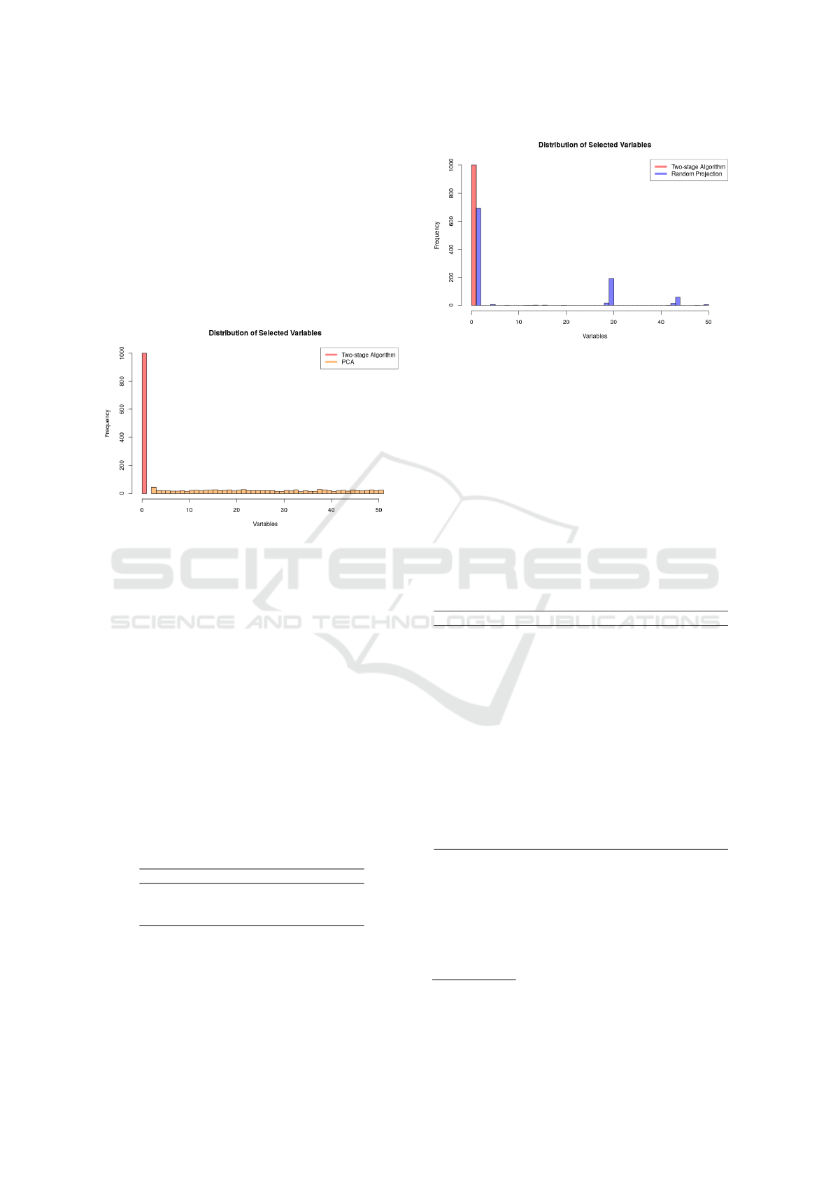
ure 1. From the histogram we can tell that projection
pursuit method select the correct variable every time
in the simulation, while PCA is tricked by the high
variance of noise terms and can never select the cor-
rect variable. While this is an overly simplified exam-
ple, we can learn from the results that PCA may not
be a reliable way of choosing parameters.
Figure 1: Distribution of selected variables. The red bars
denote weights found using two-stage projection pursuit al-
gorithm. The orange bars denote weights found using prin-
cipal component analysis.
To further emphasize the advantage of our pro-
posed two-stage projection pursuit algorithm, we con-
duct another simulation study with the same setting
as above. In stead of using PCA for dimension re-
duction, we apply the random projection pursuit by
generating 10
3
uniformly distribution random points
on the 51-dimensional unit sphere. The frequencies
of selected variables are presented in Figure 2. While
the random projection pursuit select the correct vari-
able about 60% of the time, we can tell that about 1/3
of the time it will fail such a simple task due to the
high dimension of our variable space. All above re-
sults are also summarized in Table 1.
Table 1: Counts of Selected Variables by Two-stage Projec-
tion Pursuit, Random Projection Pursuit, and PCA.
Method X
1
X
2
,. . ., X
51
Two-stage Projection Pursuit 1000 0
Random Projection Pursuit 692 308
PCA 0 1000
Figure 2: Distribution of selected variables. The red bars
denote weights found using two-stage projection pursuit al-
gorithm. The blue bars denote weights found using random
projection pursuit method.
4 DATA EXAMPLE
Bostonhousing is a popular dataset that was col-
lected by Harrison Jr and Rubinfeld (1978). In this
datset there are 13 variables that are potentially re-
lated to the housing price in Boston, and they are sum-
marized in Table 2.
Table 2: 13 Explanatory Variables and 1 Response Variable
in Boston Housing dataset.
1
Variable Description
CRIM per capita crime rate by town
ZN proportion of residential land zoned for lots
over 25,000 sq.ft.
INDUS proportion of non-retail business acres per town
CHAS Charles River dummy variable (= 1 if tract bounds river)
NOX nitric oxides concentration (parts per 10 million)
RM average number of rooms per dwelling
AGE proportion of owner-occupied units built prior to 1940
DIS weighted distances to five Boston employment centres
RAD index of accessibility to radial highways
TAX full-value property-tax rate per $ 10,000
PTRATIO pupil-teacher ratio by town
B 1000(Bk − 0.63)
2
where Bk is the proportion of blacks
by town
LSTAT % lower status of the population
MEDV Median value of owner-occupied homes in $ 1000’s
In this data example, we estimate the weight of
each of these 13 variables when fitting a linear regres-
sion model with mean absolute error (MAE). We first
compare our two-stage projection pursuit algorithm
with the first principal component. While practitioner
often use PCA as a technique for feature selection, we
1
https://archive.ics.uci.edu/ml/machine-learning-
databases/housing/
Variable Selection based on a Two-stage Projection Pursuit Algorithm
191

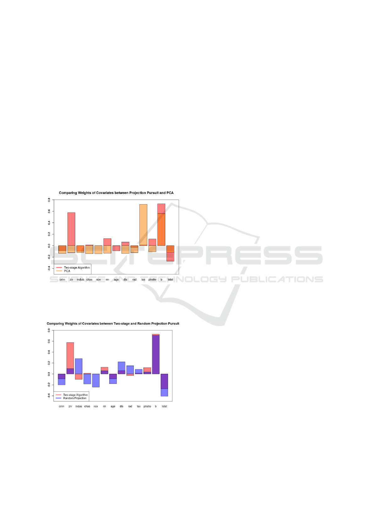
can tell from Figure 3 that the results could be very
different from projection pursuit which is specialized
in finding the optimal direction.
We further compare our results with a random
projection search by generating 10
5
uniformly dis-
tribution random points on the 13-dimensional unit
sphere. The estimated weights are presented in Fig-
ure 4. From the plot we can easily tell that there is
considerable differences for all variable weights ex-
cept one. Our explanation is that even though we
generate 10
5
uniformly distribution random points on
the 13-dimensional unit sphere, they are actually still
distributed very sparsely in the space. These random
points may not be able to cover the whole space, and
hence may very likely to miss the try direction that
will maximize our projection index which is defined
as MAE in this particular example.
Figure 3: Weight of each of 13 variables in Boston Hous-
ing dataset. The red bars denote weights found using two-
stage projection pursuit algorithm. The orange bars denote
weights found using principal component analysis.
Figure 4: Weight of each of 13 variables in Boston Housing
dataset. The red bars denote weights found using two-stage
projection pursuit algorithm. The blue bars denote weights
found using random projection pursuit method.
5 CONCLUSIONS
In this note we have introduced a new technique,
namely the two-stage projection pursuit algorithm in
achieving variable selection with high dimensional
data. We stress that PCA is based on maximizing the
proportion of total variances explained by the prin-
cipal components which may not be suitable in vari-
able selection under certain scenarios as shown un-
der our simulation studies. Projection pursuit algo-
rithm, on the other hand, can be applied to a more
flexible objective function which include PCA as a
special case. Previous efforts have been made in op-
timizing such projection indices only in lower dimen-
sional unit sphere due to computation burden. Our
proposed two-stage algorithm overcomes such limi-
tation in the optimization process within a high di-
mensional variable space. We believe this projec-
tion pursuit based method is more flexible and can
be more efficient for feature selection. In this pa-
per we used a common dataset in machine learning
to illustrate the performance of our projection pursuit
based method. Note that the proposed method can
be applied to other application settings without much
modification. Furthermore, a larger and more inten-
sive simulation study is needed to consolidate our pro-
posed method and will be included in future work.
REFERENCES
Byrd, R. H., Lu, P., Nocedal, J., and Zhu, C. (1995). A
limited memory algorithm for bound constrained op-
timization. SIAM Journal on Scientific Computing,
16(5):1190–1208.
Cadima, J., Cerdeira, J. O., and Minhoto, M. (2004). Com-
putational aspects of algorithms for variable selection
in the context of principal components. Computa-
tional statistics & data analysis, 47(2):225–236.
Cadima, J. F. and Jolliffe, I. T. (2001). Variable selection
and the interpretation of principal subspaces. Journal
of Agricultural, Biological, and Environmental Statis-
tics, 6(1):62.
Charniak, E. and Johnson, M. (2005). Coarse-to-fine n-best
parsing and maxent discriminative reranking. In Pro-
ceedings of the 43rd annual meeting on association
for computational linguistics, pages 173–180. Asso-
ciation for Computational Linguistics.
Enshaei, A. and Faith, J. (2015). Feature selection with
targeted projection pursuit. IJ Information Technology
and Computer Science, 7(5):34–39.
Friedman, J. H. and Tukey, J. W. (1974). A projection
pursuit algorithm for exploratory data analysis. IEEE
Transactions on computers, 100(9):881–890.
Harrison Jr, D. and Rubinfeld, D. L. (1978). Hedonic hous-
ing prices and the demand for clean air. Journal of
BIOINFORMATICS 2020 - 11th International Conference on Bioinformatics Models, Methods and Algorithms
192

environmental economics and management, 5(1):81–
102.
Hwang, J.-N., Lay, S.-R., Maechler, M., Martin, R. D., and
Schimert, J. (1994). Regression modeling in back-
propagation and projection pursuit learning. IEEE
Transactions on neural networks, 5(3):342–353.
Jolliffe, I. (2011). Principal component analysis. Springer.
King, J. R. and Jackson, D. A. (1999). Variable selection
in large environmental data sets using principal com-
ponents analysis. Environmetrics: The official journal
of the International Environmetrics Society, 10(1):67–
77.
Kruskal, J. B. (1972). Linear transformation of multivariate
data to reveal clustering. Multidimensional scaling,
1:101–115.
Krzanowski, W. J. (1987). Selection of variables to pre-
serve multivariate data structure, using principal com-
ponents. Journal of the Royal Statistical Society: Se-
ries C (Applied Statistics), 36(1):22–33.
Montanari, A. and Lizzani, L. (2001). A projection pursuit
approach to variable selection. Computational statis-
tics & data analysis, 35(4):463–473.
Pedersoli, M., Vedaldi, A., Gonzalez, J., and Roca, X.
(2015). A coarse-to-fine approach for fast deformable
object detection. Pattern Recognition, 48(5):1844–
1853.
Variable Selection based on a Two-stage Projection Pursuit Algorithm
193