
What Does Multi-agent Path-finding Tell Us About Intelligent
Intersections
V
ˇ
era
ˇ
Skopkov
´
a, Roman Bart
´
ak
a
and Ji
ˇ
r
´
ı
ˇ
Svancara
b
Charles University, Faculty of Mathematics and Physics, Prague, Czech Republic
Keywords:
Multi-agent Systems, Centralized Planning, Cooperative Navigation, Intelligent Intersection.
Abstract:
In this paper, we study the problem of an intelligent intersection. There are many studies that present an
algorithm that tries to efficiently coordinate many agents in a given intersection, however, in this paper, we
study the layout of the intersection and its implications to the quality of the plan. We start with two of today
commonly used road intersections (4-way intersection and roundabout) and compare them with an intersection
that is less restrictive on the movements of the agents. This means that the agents do not have to use predefined
lanes or follow a prescribed driving direction. We also study the effect of granularity of the intersection. The
navigation of the agents in a given intersection is solved as an instance of (online) multi-agent path-finding
problem.
1 INTRODUCTION
Intersections are nowadays one of the most problem-
atic parts of our roads. According to the statistics
(Huang et al., 2008), intersections are the place where
most accidents happen. Navigating through an inter-
section is problematic because the paths of the vehi-
cles cross each other and so not all vehicles can move
at the same time. This means that some vehicles must
stand still and yield the others. If the traffic around
the intersection is dense enough, then a situation can
happen when every newly arriving vehicle must spend
more and more time waiting to get through the inter-
section.
In order to make the intersection effective, and
above all safe, various intersection management
mechanisms have been utilized. In low-traffic inter-
sections, following the traffic regulations and respect
the traffic signs is enough. In busier intersections, we
encounter traffic lights that can control traffic in all
directions. However, these mechanisms are not effi-
cient. For example, if we arrive at an empty intersec-
tion but have a red light, we must not continue our
journey, although there is no one to whom we are giv-
ing way. In this case, the light signal control does not
behave optimally at all, because otherwise, it would
recognize that we are alone at the intersection and let
us through.
a
https://orcid.org/0000-0002-6717-8175
b
https://orcid.org/0000-0002-6275-6773
If we take into account the rise of autonomous ve-
hicles, we can further develop the idea of an intelli-
gent intersection in such a way that it can communi-
cate with the vehicles that want to go through. Instead
of the intersection recognizing a vehicle and changing
lights, the vehicle asks for permission to pass through
the intersection at a given time and the intersection
navigates it safely with other present vehicles.
Note that while we are using the terminology from
car navigation, the same problems can be found in
other areas of agent navigation. For example ware-
house robots – navigation between shelves, where
movement in only one direction is allowed, is easy
using only sensors. However, navigation through a
crossing of these corridors is hard due to the presence
of other robots. Some other examples include ship
navigation within harbors in comparison with naviga-
tion on the open sea, and airplane navigation in the
proximity to an airport with comparison to flights in
predefined flight corridors. For this reason, we will
use the more general term agents.
Several studies present an algorithm that navigates
agents through a fixed intersection. In contrast, we
will study the effect of the layout of the intersection
on the quality of plans. The intersections can be ab-
stracted as a shared graph and the navigation part is
then solved as an instance of multi-agent path-finding
(MAPF) problem.
250
Škopková, V., Barták, R. and Švancara, J.
What Does Multi-agent Path-finding Tell Us About Intelligent Intersections.
DOI: 10.5220/0009098502500257
In Proceedings of the 12th International Conference on Agents and Artificial Intelligence (ICAART 2020) - Volume 1, pages 250-257
ISBN: 978-989-758-395-7; ISSN: 2184-433X
Copyright
c
2022 by SCITEPRESS – Science and Technology Publications, Lda. All rights reserved

2 MAPF PROBLEM
Offline MAPF. An instance of offline MAPF problem
can be formally defined as a pair (G, A), where G is a
graph and A is a set of agents. The graph G can be di-
rected or undirected. Each agent a ∈ A is defined as a
pair (a
s
, a
g
), where a
s
and a
g
correspond to a starting
location and goal location respectively in graph G.
The time is assumed discretized and in each
timestep, all of the agents can perform either a move
action to one of the neighboring vertices or a wait ac-
tion to remain in the current vertex. All of the agents
are moving simultaneously.
A plan for a single agent i is a sequence of loca-
tions where the agent is located at a given time. Let π
i
denote a plan for agent i, where π
i
( j) = v represents
that agent i is located in vertex v at timestep j. We
denote |π
i
| as the length of the plan.
A plan π
i
is a valid plan if π
i
(0) and π
i
(|π
i
|) are
the initial and goal locations of a
i
, respectively, and
for every j ∈ {0, . . . , |π
i
|} either π
i
( j) = π
i
( j + 1)
or (π
i
( j), π
i
( j + 1)) ∈ E. This means that at each
timestep, the agent is either waiting in the current ver-
tex or moves to a neighboring vertex.
A joint plan π is a set of valid plans, one for each
agent. The joint plan must further satisfy the follow-
ing constraints:
• ∀i, j ∈ A, ∀t : π
i
(t) 6= π
j
(t) Meaning that no two
agents can occupy the same vertex at the same
time.
• ∀i, j ∈ A, ∀t : π
i
(t) 6= π
j
(t + 1) ∨ π
i
(t + 1) 6= π
j
(t)
Meaning that no two agents can use the same edge
in the opposite direction at the same time.
In the context of MAPF, we call these constraints a
vertex conflict and a swapping conflict (Stern et al.,
2019). On the other hand, we allow two agents to
closely follow each other. This means that agent a can
move into a vertex that is currently occupied by some
other agent, provided that the vertex will be empty be-
fore the arrival of the agent a. This situation is for ex-
ample forbidden in the setting of MAPF that is called
Pebble Motion (Kornhauser et al., 1984).
When creating a plan, we often prefer to find
an optimal plan with respect to some cost function.
The two functions often used in the literature are
makespan and sum of costs.
The makespan function is defined as:
max
i∈A
|π
i
|
The sum of costs function is defined as:
∑
i∈A
|π
i
|
While there are many polynomial-time algorithms
that can find a feasible solution (de Wilde et al., 2014;
Surynek, 2009), the task to find either a makespan op-
timal solution or a sum of costs optimal solution is
an NP-Hard problem (Ratner and Warmuth, 1990; Yu
and LaValle, 2013).
Online MAPF. As opposed to the offline setting,
where all of the agents are known in advance, we
can define an online MAPF (
ˇ
Svancara et al., 2019),
where new agents can appear over time, while agents
that reached their goal location disappear. This set-
ting very closely represents the intersection model we
are interested in.
Formally an online MAPF instance includes in ad-
dition to the offline instance a set of new agents A
new
.
Each new agent a is a triple (a
s
, a
g
, t), where t is the
timestep at which the agent wants to enter the graph.
If it is not possible for the agent to enter at the desired
time (because it would cause an unavoidable colli-
sion), it is possible to delay the agent.
The solution to the online MAPF is then a se-
quence of valid joint plans Π = (π
0
, . . . , π
m
), where
m = |A
new
| and π
0
is the joint plan for the offline part
of the instance. Each time a new agent enters the
graph, we produce a new plan including that agent.
Depending on the solver strategy, we may forbid or
allow to change plans for the agents that were already
present in the graph.
Note that the online nature of the problem means
that there is no solver that can compute the overall
optimal solution (
ˇ
Svancara et al., 2019).
3 INTERSECTION MODEL
An intersection is a part of a shared environment
where several roads with simple navigation rules
cross each other. Intersections are typically hard for
agents to navigate through due to the presence of
many other agents, whose desired paths cross each
other.
A way to deal with this challenge is for the agents
to be coordinated by some centralized autonomous in-
tersection management that organizes the agents in
such a way that they do not collide and, furthermore,
the time spend crossing the intersection is minimized
(Dresner and Stone, 2008b). There are some ba-
sic logical requirements for this intersection manage-
ment such as that all of the independent agents (driver
agent) respect the commands of the central agent (in-
tersection manager). For simplicity, we assume that
all of the driver agents are homogeneous and are trav-
elling at the same speed.
What Does Multi-agent Path-finding Tell Us About Intelligent Intersections
251
The intersection is characterized by some loca-
tions, where an agent can enter and some locations
where the agent may leave the intersection. Once the
agent leaves the intersection, it is again an indepen-
dent agent.
The driver agents send a request for traversing the
intersection with the desired entrance time and trajec-
tory. The intersection manager then either approves
or rejects this request. A simple strategy to coordinate
the intersection can be described as first-come, first-
served (Dresner and Stone, 2008b). In this strategy,
the intersection manager simply checks if the request
can be executed without causing a collision with pre-
viously approved trajectory and if so it approves the
request.
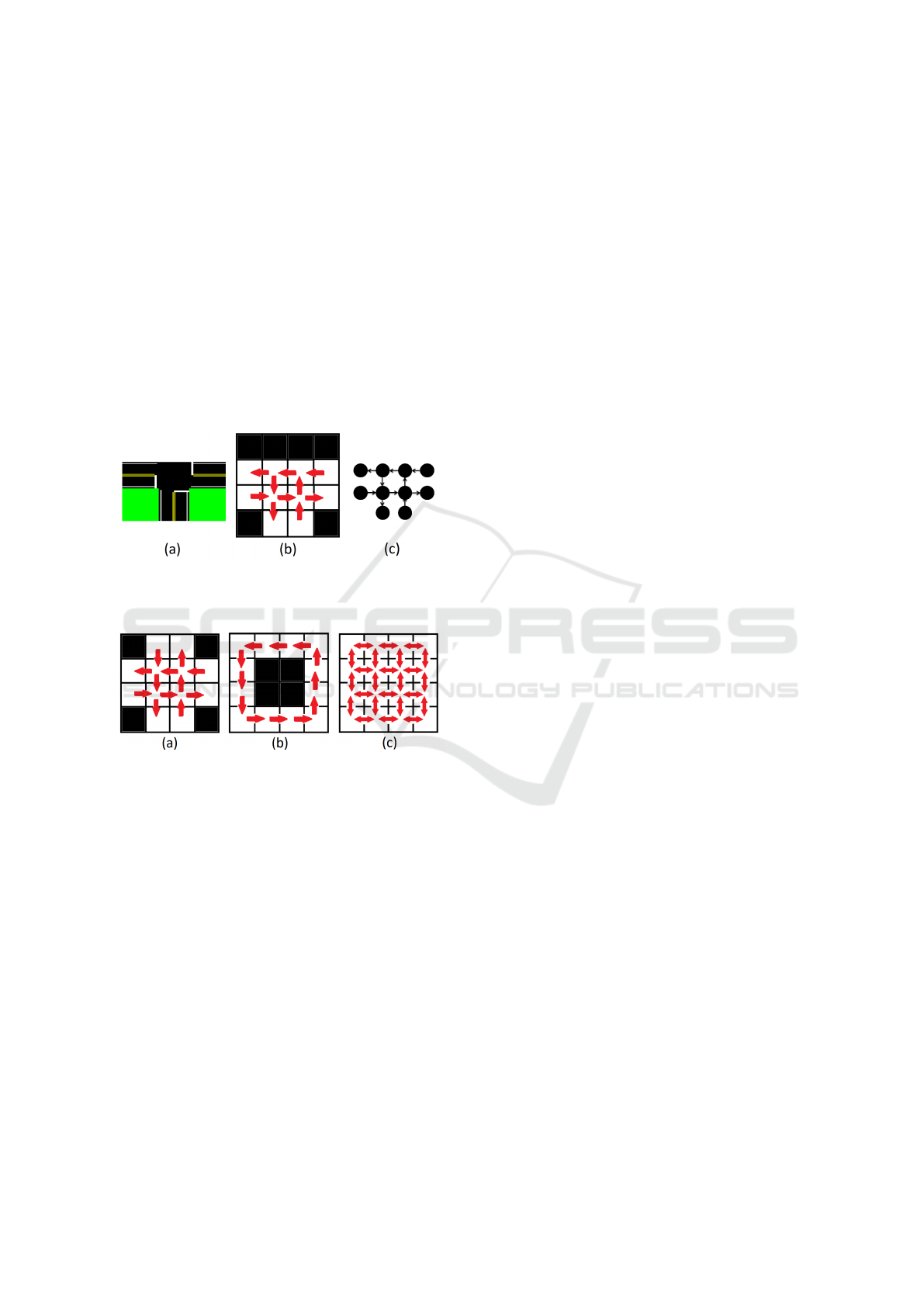
Figure 1: The process of creating an input graph for MAPF
from real intersection: (a) real intersection (b) tiles repre-
sentation (c) oriented graph.
Figure 2: Intersection types: (a) corridors intersection (b)
roundabout intersection (c) free movement intersection.
In this paper, we try to improve the intersection man-
ager by letting it decide the trajectory of the agent.
We will also consider a model, where the intersection
manager can change the already approved trajectories
of the agents that are already traversing the intersec-
tion. This approach can be used also for emergencies
when an accident happens in the intersection and we
need to change the approved trajectories to avoid the
collision (Dresner and Stone, 2008a).
4 COORDINATING
INTERSECTION USING MAPF
Intersection Representation. We divide the space of
the intersection into a grid of n × n tiles, we call n the
granularity of the intersection. In every timestep, an
agent can occupy only one tile and a tile can be occu-
pied by at most one agent. We suppose that the agents
move synchronously and in every discrete timestep
they move to one of their neighboring tiles, they are
not allowed to stay on the same tile in two consequent
timesteps (wait actions are not allowed).
Every tile has at most 4 neighboring tiles —- they
can be situated to the north, to the south, to the east
and to the west of that tile. The diagonal tiles are not
neighbors. The space of the intersection is described
as a graph in this way: The tiles correspond to the ver-
tices of the graph and the edges represent all couples
of the neighboring edges. An example of translating a
real intersection into tiles representation and then into
oriented graph representation can be seen in Figure 1.
Then we can apply MAPF on this graph in order to
find paths for agents in the intersection. We reduced
the intersection manager to an online MAPF problem.
A tile might have less than 4 neighbors because
of two reasons. Firstly, edge tiles do not have natu-
rally some neighbors because they simply do not ex-
ist. Secondly, it may be forbidden to perform some
moves in the intersection. This can be achieved by
forbidding a tile to be a neighbor of any other tile by
deleting an appropriate edge from the graph. If the
edge is completely missing, two tiles are not neigh-
boring although they lay physically next to each other.
In case there is a directed edge between two tiles, it is
possible to move between these tiles in the direction
of that edge, but movement in the opposite direction
is forbidden.
Intersection Models. We created three different in-
tersection types to compare (see Figure 2). Two of
them are a sample of intersections used in the real
world, while the last one gives the agents more free-
dom in movement.
The Corridors Intersection is represented by a di-
rected graph. Its edges limit the movement of the
agents through the intersection in such a way that the
trajectories approximately correspond to those which
a human driver would choose. This is a representation
of a typical 4-way intersection that is usually coordi-
nated by traffic lights or by signs.
The Roundabout Intersection is also represented
by a directed graph. It simulates a roundabout build
on the space reserved for the intersection —- it is of
the same size but it allows only the movement through
the margin tiles of the intersection in the counter-
clockwise direction. The tiles in the middle of the
intersection are unreachable.
The Free Movement Intersection is represented by
an undirected graph. It contains an undirected edge
between each couple of tiles laying next to each other.
ICAART 2020 - 12th International Conference on Agents and Artificial Intelligence
252
The two previous intersections are used today in traf-
fic because a few simple rules can achieve coordinated
movement of agents inside the intersection. The free
movement intersection, on the other hand, is not vi-
able to use without some centralized entity that coor-
dinates the movement of agents. The benefit of this
intersection is that it allows the agents to move freely
through the whole space of the intersection, thus the-
oretically increasing throughput.
Incoming Requests. Every request consists of in-
put and output direction and of the required time (in
abstract discrete units) for entering the intersection.
Before every experiment, we always set the space
limit – maximum delay allowed on every entrance
to the intersection. Requests for which there is no
free path starting between required time and (required
time + maximum delay) are rejected.
Solvers. We always process one new request in one
run of the solver although it is possible to process
more requests at once. In most cases, we search
path for a new request in such a way that we re-
spect the found paths for all previous requests and
we do not change them. We shall call this approach
adding-solver. In some experiments we use also
rescheduling-solver which, in contrast to the previ-
ous one, also might change some paths found before.
Such solver is more powerful — it might succeed in
some cases in which the adding-solver fails but its
computations may take a longer time.
We should mention that it is reasonable to use
rescheduling-solver only for the model of free move-
ment intersection. In the rest of the models there is
always only one possible path in every direction, no
alternative paths exist. Then the rescheduling of pre-
vious agents does not bring us any new information.
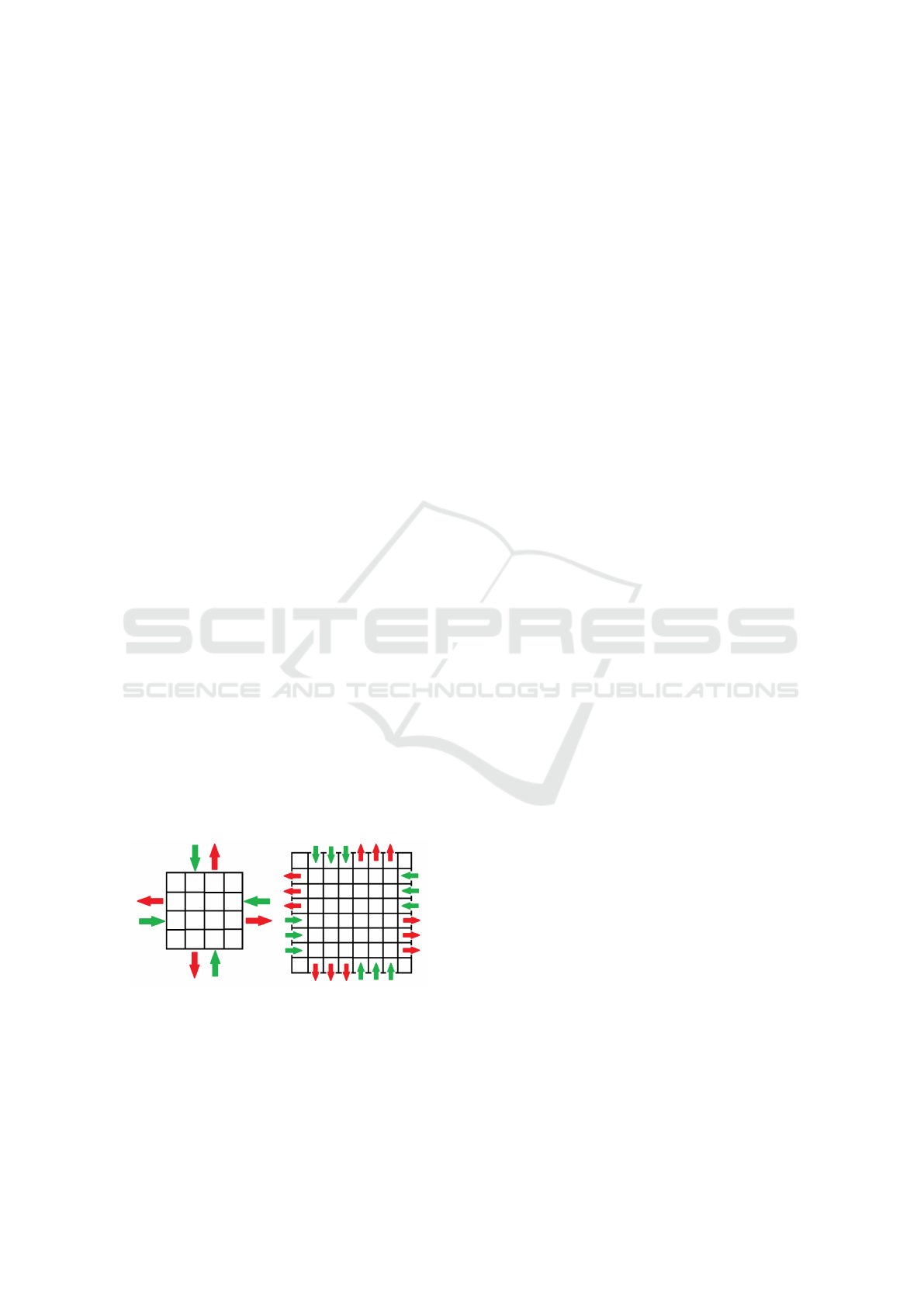
Figure 3: Input tiles for intersections with granularities
n = 4 and n = 8.
Experimental Settings. In our experiments we use
two granularities: n = 4 and n = 8. For n = 4 we have
one input tile and one output tile for every direction,
for n = 8 we chose to have 3 input tiles and 3 output
tiles in every direction (see Figure 3). In this case, we
allow the agents to use arbitrary input and output tile
in a requested direction. The requests do not corre-
spond to a particular tile, only to directions. Specific
tiles for every agent are chosen by the solver.
Since there are more options for the agents to en-
ter the graph in the 8 by 8 grid, there are more possi-
bilities of how to define the corridors in the intersec-
tion (see Figure 4). We can either forbid to change
lines once the agent enters the intersection or we can
allow it. If the line switching is forbidden then one
input tile corresponds exactly to one output tile, thus
the agent is forced to enter the graph based on the
desired output direction (Figure 4 (a)). On the other
hand, if we allow the agent to change lines, the solver
has more choices where the agent can enter (Figure
4 (b)). We can increase the number of choices even
more by allowing the agents to move even over the
input tiles (Figure 4 (c)). Note that the version (c) has
still only three input and output tiles in each direction.
Also, there is a difference between corridor versions
(b) and (c), and the free movement intersection. The
free movement intersection allows movement in every
direction, while the corridor intersection only allows
movement in up to two directions in any given tile.
Increasing the granularity does not change the in-
ternal structure of the roundabout intersection and
free movement intersection.
5 EXPERIMENTS
In this section, we describe experiments in which
we tested the performance of our models at differ-
ent levels of traffic density. For every experiment, we
generated 5 random sequences of input requests cor-
responding to parameters stated before and we pro-
cessed them by tested intersections. Every sequence
was characterized by minimum and maximum num-
ber of requests which could appear in every discrete
timestep, by the timestep in which the last request
came and by space limit used.
To generate the requests we used a generator with
uniform distribution. At first we always randomly
chose the number of requests for a timestep (within a
given range) and then we generated input and output
direction for particular requests independently. The
only condition was that the directions can not be equal
(we do not support the so-called U-turns).
Since it is not important how a particular instance
of a MAPF problem is solved, we do not describe in
much detail the MAPF solver that was used in the ex-
periments. The solver is based on reducing the in-
stance into a satisfiability problem using the declar-
What Does Multi-agent Path-finding Tell Us About Intelligent Intersections
253
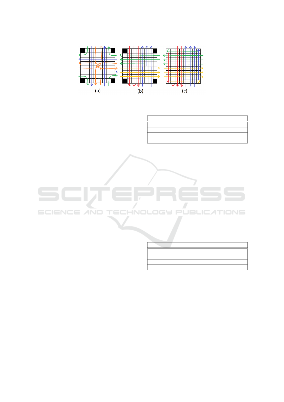
Figure 4: Three different line settings in the 8 × 8 corridor intersection. (a) strict lines (b) free lines (c) oriented graph.
ative language Picat (Bart
´
ak et al., 2017). In the
adding-solvers, we always compute a path for only
one agent (while avoiding the planned agents), thus
it is the problem of finding the shortest path. In the
rescheduling-solver, we find the makespan optimal
solution.
In our tables we always present averages of results
of 5 inputs generated with equal parameters. There
are three metrics we are interested in:
Plan Length corresponds to the number of discrete
timesteps needed to transport all agents to their goals
according to the plan. We measure the experiment
from time 1.
Delay is the cumulative number of timesteps each
agent has to spend in the intersection (or waiting
before entering the intersection) over the minimum
number of timesteps it would take the agent to reach
the goal position if there were no other agents present.
Refused is the number of requests which were not
possible to plan within a given space-limit. The re-
quests that were refused did not move through the in-
tersection at all.
Light Traffic. In the first experiment, we worked
with intersections with granularity n=4. Tested input
sequences consisted of exactly one request in every
timestep which corresponded to light traffic situation.
The space limit was set to 1.
We tested all three models in connection with
adding-solver, the free movement intersection model
was tested also together with rescheduling-solver.
The results of this experiment are noted in table 1.
Almost every request in every model was accepted,
the only model which refused some requests was the
corridors model. The plan of the roundabout model
was a bit longer than the other plans but the difference
was not considerable.
The free movement intersection model had a
smaller delay than the corridors model, the best result
was achieved by free movement intersection model
together with rescheduling solver. It means in some
situations there existed a better solution than the one
Table 1: Results for light traffic with space limit of 1.
Intersection type plan length delay refused
Roundabout 15.6 1 0
Corridor 13 2.4 0.2
Free – adding 13 1.4 0
Free – rescheduling 13 0.8 0
adding-solver found but it had required a change of
the plan of some agent(s) planned before.
Medium Traffic. In this experiment, we use the
same parameters except that there can be from 0 to 2
requests in every timestep. Generated sequences rep-
resent medium traffic density.
The results of this experiment are summarized
in table 2. The most successful model was the
model of free movement intersection, this time in
connection with adding-solver. It happened be-
cause rescheduling-solver time-outed on some re-
quests, otherwise it should always find at least the
same results as adding-solver.
Table 2: Results for medium traffic with space limit of 1.
Intersection type plan length delay refused
Roundabout 20.2 2.4 0.8
Corridor 17.2 4.4 1.6
Free – adding 17.4 5.8 0.4
Free – rescheduling 18 4.75 1
As in the previous example, the plan length of the
roundabout model is worse in comparison with the
rest of the models. But we should notice that the de-
lay of this model was the smallest of all models.
Since the rescheduling-solver tends to time-out,
we will no longer consider it in further experiments.
The experiments will increase in difficulty and the
trend of time-outing will be more prominent. The
intersection management should be a fast responding
entity, the agent can not afford to wait several minutes
before receiving approval to enter the intersection.
ICAART 2020 - 12th International Conference on Agents and Artificial Intelligence
254
Heavy Traffic. In this example, there will be heavy
traffic consisting of 1 to 3 requests in every timestep.
We can expect a bigger number of refused requests.
We run the testing input sequences twice. First,
there will be a space limit of 1, in the second run space
limit will be 5.
The results of both variants of this experiment are
compared in tables 3 and 4. In both cases, we can see
that free movement intersection refused the smallest
number of agents. With the space limit of 1, there
was a shorter plan length and smaller delay when us-
ing the corridor model. But we should mention that
this number is influenced by the fact that some agents
were refused so the resulting plan of corridor model
is in reality simpler.
Table 3: Results for heavy traffic with space limit of 1.
Intersection type plan length delay refused
Roundabout 18.4 5.2 4.2
Corridor 14 8.4 3.4
Free 15 10.8 2
Table 4: Results for heavy traffic with space limit of 5.
Intersection type plan length delay refused
Roundabout 18.8 20 0.6
Corridor 16.4 31.4 0.4
Free 15.4 19.2 0
When comparing both tables we can notice that with
increasing space limit, the number of refused agents
decreases and the delay increases. The length of the
plan stays almost the same. Higher space limit adds
flexibility to solver so it is able to schedule some ex-
tra agents but there is no other possibility than to de-
lay their starts so the delay increases rapidly (almost
twice).
Extremely Heavy Traffic. In the following experi-
ment, we have extremely heavy traffic consisting of 2
to 5 requests in every timestep. At first, we allow only
a space limit of 2, later we increase it to 5. We expect
there will be a huge number of refused requests and
the majority of the others will have big delays.
Results of this experiment are available in tables
5, 6. In both cases we can see similar results as in
previous experiments: free movement intersection re-
fused the fewest requests and the roundabout model
had the largest plan length.
When comparing both tables we can notice that
with a space limit of 5 there is a significant decrease
in the number of refused requests. Since the length of
the plan stayed almost the same, it means the space of
the intersection is better utilized.
Table 5: Results for extremely heavy traffic with space limit
of 2.
Intersection type plan length delay refused
Roundabout 17.2 15 8.2
Corridor 14 21.4 9.6
Free 14.8 36.2 5.8
Table 6: Results for extremely heavy traffic with space limit
of 5.
Intersection type plan length delay refused
Roundabout 19 47 3.6
Corridor 17 59.2 3.8
Free 16.2 63.6 1.6
Unfortunately with a space limit of 5, the delay in-
creased considerably which was caused mainly be-
cause of the additional space limit. We can observe
it in the results of the roundabout model. With the
space limit of 2, there was only 15 timesteps delay in
this model. But with the space limit of 5, it increased
to 47. Since there are no alternative (and longer) paths
in the roundabout model the value of the delay in this
model consists only of waiting in front of the intersec-
tion. Thus on average, in the intersection with space
limit of 5 an agent waits in front of the intersection
three times longer than in the intersection with space
limit of 2.
It means that if we want the solver to accept as
many requests as possible and to plan their paths with
minimum delay all at once, we have to reach a com-
promise.
Long-term Extremely Heavy Traffic. In this ex-
periment, we will simulate the situation of an arising
traffic jam. Every timestep there will be between 2
and 5 requests and the experiment will run 3 times
longer than all previous experiments. Only free move-
ment intersection will be tested and there will be two
runs of the experiment - with a space limit of 2 and 5.
The results of this experiment can be seen in table
7. When using the space limit of 5, there were ac-
cepted 2 more agents but otherwise, the result is not
very successful. The delay increased more than twice
which is quite unsatisfying.
Table 7: Results for long-term extremely heavy traffic over
the free-movement intersection solved by the adding-solver.
Space limit plan length delay refused
2 36 169 32
5 40 350 30
Figure 5 shows the number of refused requests in ev-
What Does Multi-agent Path-finding Tell Us About Intelligent Intersections
255
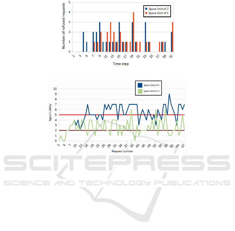
Figure 5: Number of refused requests in individual timesteps in long-term extremely heavy traffic.
Figure 6: Delay of particular agents in long-term extremely heavy traffic.
ery timestep. We can see that there were 2 requests
refused in space limit of 2 before refusal of the first
request in space limit of 5. The reason for that was
probably the size of the space limit — a smaller time
window was filled up sooner so the solver had to start
refusing the requests sooner. After a 5-step window
was filled up the number of refused requests was al-
most the same.
In the figure 6 we can observe the origin of the
traffic jam. A few agents at the beginning have just
small delays but quickly the majority of agents start
to have delay approximately the size corresponding to
the relevant space limit. This means that the majority
of agents are planned at the end of the allowed time
window, almost none of them were planned at their
required time.
We can conclude that in the longer horizon, a big-
ger space limit does not increase the throughput of
the intersection, in contrast, it only delays particular
agents more. On average, an agent has a 2.5 step de-
lay in plan with a space limit of 2 while it has a 5.1
step delay in plan with a space limit of 5.
By increasing the space limit we slightly post-
poned the formation of the traffic jam but we had not
avoided it. So it is reasonable to use a small space
limit to increase the throughput of the intersection.
Intersection 8 × 8. In the last experiment, we use
intersection with granularity n = 8 and we test several
corridor models which we compare with free move-
ment intersection.
After extending the corridor model to an intersec-
tion with higher granularity, we can observe two inter-
esting issues. At first such an intersection should have
more than one input and output tiles for every direc-
tion, otherwise, input tiles would be a bottleneck of
the intersection. Furthermore, if we model corridors
in a bigger intersection we can have separate lanes for
particular directions.
In our experiment, we use 3 input and output tiles
for every direction and 3 different types of corridor
model described before.
The results of this experiment are described in ta-
ble 8. The models are ordered from the most restric-
tive to the most liberal one in the table. The number
of refused agents corresponds to this ordering, more
liberal models refused fewer agents. The length of
the plan is almost equal, the most interesting metric
in this experiment is the delay.
The smallest delay had the model of strict lines
corridor. It was because its graph has almost no alter-
native paths and thus the planned paths are optimal.
An interesting result is that the free lines corridor has
ICAART 2020 - 12th International Conference on Agents and Artificial Intelligence
256

a bigger delay although it has an equal number of re-
fused requests. It is probably the result of freedom
which was given to the model, it used some unsuit-
able paths in the beginning and then the other agents
had to wait in front of the intersection.
Table 8: Results for 8×8 intersections based on different
line management.
Intersection type plan length delay refused
Corridor – strict lines 17.8 12.4 1.2
Corridor – free lines 18.5 15.8 1.2
Corridor – oriented graph 18.4 17 1
Free 17.6 13 0
6 CONCLUSION
In this paper, we studied an intelligent intersection
design. The intersection manager receives requests
for traversing the shared environment and its job is
to navigate all of the agents through the intersection
safely and as efficiently as possible.
Rather than an algorithm that plans and schedules
the paths itself, we studied the spatial design of the in-
tersection and its effect on the efficiency of the found
plan. The planning itself can be seen as an instance
of multi-agent path-finding. We assumed two types of
intersections that are commonly used on roads today -
4-way intersection with turning lanes and roundabout.
We also added an intersection with less restriction on
the movements, where agents can travel in any direc-
tion.
The extensive simulation experiments show that
while roundabout type intersections do not cause
much extra delay to the agents, the traversed path is
quite long in comparison with other types. The free
movement type intersection has the highest through-
put of the agents at the expense of higher delay. This
is caused by the higher flexibility of the paths the
agents can traverse. If the optimal path in the re-
stricted intersection is occupied, the agent has to wait,
however, in the free movement intersection, the agent
can still find some less optimal path to go through.
ACKNOWLEDGEMENTS
This research is supported by the Czech Science
Foundation under the project P103-19-02183S, by
SVV project number 260 453, and by the Charles
University Grant Agency under the project 90119.
REFERENCES
Bart
´
ak, R., Zhou, N., Stern, R., Boyarski, E., and Surynek,
P. (2017). Modeling and solving the multi-agent
pathfinding problem in picat. In 29th IEEE Interna-
tional Conference on Tools with Artificial Intelligence,
ICTAI 2017, Boston, MA, USA, November 6-8, 2017,
pages 959–966.
de Wilde, B., ter Mors, A., and Witteveen, C. (2014). Push
and rotate: a complete multi-agent pathfinding algo-
rithm. J. Artif. Intell. Res., 51:443–492.
Dresner, K. M. and Stone, P. (2008a). Mitigating catas-
trophic failure at intersections of autonomous vehi-
cles. In 7th International Joint Conference on Au-
tonomous Agents and Multiagent Systems (AAMAS
2008), Estoril, Portugal, May 12-16, 2008, Volume 3,
pages 1393–1396.
Dresner, K. M. and Stone, P. (2008b). A multiagent ap-
proach to autonomous intersection management. J.
Artif. Intell. Res., 31:591–656.
Huang, H., Chin, H. C., and Haque, M. M. (2008). Severity
of driver injury and vehicle damage in traffic crashes
at intersections: A bayesian hierarchical analysis. Ac-
cident Analysis & Prevention, 40(1):45 – 54.
Kornhauser, D., Miller, G. L., and Spirakis, P. G. (1984).
Coordinating pebble motion on graphs, the diame-
ter of permutation groups, and applications. In 25th
Annual Symposium on Foundations of Computer Sci-
ence, West Palm Beach, Florida, USA, 24-26 October
1984, pages 241–250.
Ratner, D. and Warmuth, M. K. (1990). Nxn puzzle
and related relocation problem. J. Symb. Comput.,
10(2):111–138.
Stern, R., Sturtevant, N. R., Felner, A., Koenig, S., Ma, H.,
Walker, T. T., Li, J., Atzmon, D., Cohen, L., Kumar,
T. K. S., Boyarski, E., and Bart
´
ak, R. (2019). Multi-
agent pathfinding: Definitions, variants, and bench-
marks. In the International Symposium on Combina-
torial Search (SoCS).
Surynek, P. (2009). A novel approach to path planning
for multiple robots in bi-connected graphs. In 2009
IEEE International Conference on Robotics and Au-
tomation, ICRA 2009, Kobe, Japan, May 12-17, 2009,
pages 3613–3619.
ˇ
Svancara, J., Vlk, M., Stern, R., Atzmon, D., and Bart
´
ak,
R. (2019). Online multi-agent pathfinding. In The
Thirty-Third AAAI Conference on Artificial Intelli-
gence, AAAI 2019, The Thirty-First Innovative Ap-
plications of Artificial Intelligence Conference, IAAI
2019, The Ninth AAAI Symposium on Educational
Advances in Artificial Intelligence, EAAI 2019, Hon-
olulu, Hawaii, USA, January 27 - February 1, 2019.,
pages 7732–7739.
Yu, J. and LaValle, S. M. (2013). Structure and intractability
of optimal multi-robot path planning on graphs. In
Proceedings of the Twenty-Seventh AAAI Conference
on Artificial Intelligence, July 14-18, 2013, Bellevue,
Washington, USA.
What Does Multi-agent Path-finding Tell Us About Intelligent Intersections
257
