Heavy Caterpillar Distances for Rooted Labeled Unordered Trees

Nozomi Abe, Takuya Yoshino and Kouich Hirata

Kyushu Institute of Technology, Kawazu 680-4, Iizuka 820-8502, Japan

Keywords:

Heavy Caterpillar, Heavy Caterpillar Distance, Rooted Labeled Unordered Tree, Tree Edit Distance, Varia-

tions of Tree Edit Distance.

Abstract:

In this paper, we introduce two heavy caterpillar distances between rooted labeled unordered trees (trees, for

short) based on the edit distance between the heavy caterpillars obtained from the heavy paths in trees. Then,

we show that the heavy caterpillar distances provide the upper bound of the edit distance for trees, can be

computed in quadratic time under the unit cost function and are incomparable with other variations of the edit

distance.

1 INTRODUCTION

Comparing tree-structured data such as HTML and

XML data for web mining or RNA and glycan data for

bioinformatics is one of the important tasks for data

mining. The most famous distance measure (Deza

and Deza, 2016) between rooted labeled unordered

trees (trees, for short) is the edit distance τ

TAI

(Tai,

1979). The edit distance is formulated as the mini-

mum cost of edit operations, consisting of a substitu-

tion, a deletion and an insertion, applied to transform

a tree to another tree. It is known that the edit distance

is always a metric and coincides with the minimum

cost of Tai mappings (Tai, 1979). Unfortunately, the

problem of computing the edit distance between trees

is MAX SNP-hard (Zhang and Jiang, 1994). This

statement also holds even if trees are binary or the

maximum height of trees is at most 3 (Akutsu et al.,

2013; Hirata et al., 2011).

Many variations of the edit distance have de-

veloped as more structurally sensitive distances as

the minimum cost of the variations of the Tai map-

ping (Jiang et al., 1995; Kan et al., 2014; Kuboyama,

2007; Lu et al., 2001; Wang and Zhang, 2001; Ya-

mamoto et al., 2014; Yoshino and Hirata, 2017;

Zhang, 1996). In particular, the alignment distance

ALN

(Jiang et al., 1995) and the segmental distance

(Kan et al., 2014) are the most general variations

of τ

TAI

, where τ

ALN

is incomparable with τ

, and

the isolated-subtree distance τ

ILST

(Wang and Zhang,

2001) (or constrained distance) (Zhang, 1996) is the

most general tractable variation of τ

TAI

(Yoshino and

Hirata, 2017).

A caterpillar (cf. (Gallian, 2007)) is a tree trans-

formed to a path after removing all the leaves in it.

Recently, Muraka et al. (Muraka et al., 2018) have

shown that the problem of computing the edit distance

between caterpillars is tractable and the structural re-

striction of caterpillars provides the limitation of the

tractability for computing the edit distance. Also Mu-

raka et al. (Muraka et al., 2019) have developed the

method to fast approximate the edit distance between

caterpillars.

Hence, in this paper, we introduce new distances

for trees by using the edit distance between the em-

bedded caterpillars. Then, we focus on the heavy

path (Sleator and Tarjan, 1983), which is a famous

embedded path in a tree obtained by selecting vertices

whose number of descendants is largest from the root.

In particular, Demaine et al. (Demaine et al., 2009)

have adopted the heavy path to analyze the time com-

plexity of computing the edit distance for rooted la-

beled ordered trees.

In this paper, ﬁrst we formulate a heavy caterpil-

lar in a tree as the caterpillar whose backbone is the

heavy path in the tree and whose set of leaves con-

sists of all the adjacent vertices to the heavy path in

the tree. Then, we introduce the following two heavy

caterpillar distances τ

and τ

between trees.

The heavy caterpillar distance τ

is formulated

as the sum of the edit distance between heavy cater-

pillars and the cost of deleting and inserting the re-

mained vertices not contained in the heavy caterpil-

lars. On the other hand, the heavy caterpillar distance

is formulated as the sum of the edit distance be-

tween heavy caterpillars and the cost of the Tai map-

198

Abe, N., Yoshino, T. and Hirata, K.

Heavy Caterpillar Distances for Rooted Labeled Unordered Trees.

DOI: 10.5220/0009095801980204

In Proceedings of the 9th International Conference on Pattern Recognition Applications and Methods (ICPRAM 2020), pages 198-204

ISBN: 978-989-758-397-1; ISSN: 2184-4313

ping obtained by repeating recursively, after selecting

vertices (as leaves in heavy caterpillars) to bridge the

Tai mapping between the heavy caterpillars, to com-

pute the edit distance (the Tai mapping) between the

heavy caterpillars of the complete subtree rooted by

the selected vertices.

Then, in this paper, we show that the heavy cater-

pillar distances τ

and τ

provide the upper bound

of τ

TAI

, that is, τ

TAI

≤ τ

. For the maxi-

mum height h and the maximum number λ of leaves

in given two trees, we can compute τ

in O(h

)

time under the general cost function and in O(h

λ)

time under the unit cost function, and τ

) in

O(h

) time under the general cost function and in

O(h

) time under the unit cost function. Further-

more, we show that τ

and τ

are incomparable

with τ

ILST

, τ

ALN

and τ

. Hence, the heavy caterpillar

distances τ

and τ

provide another tractable vari-

ations of the edit distance τ

TAI

incomparable with the

isolated-subtree distance τ

ILST

2 PRELIMINARIES

A tree T is a connected graph (V,E) without cycles,

where V is the set of vertices and E is the set of edges.

We denote V and E by V(T) and E(T). The size of

T is |V| and denoted by |T|. We sometime denote

v ∈ V(T) by v ∈ T. We denote an empty tree (

0) by

0. A rooted tree is a tree with one node r chosen as its

root. We denote the root of a rooted tree T by r(T).

Let T be a rooted tree such that r = r(T) and

u, v, w ∈ T. We denote the unique path from r to v, that

is, the tree (V

′

) such that V

′

= {v

,... , v

}, v

= r,

= v and (v

i+1

) ∈ E

′

for every i (1 ≤ i ≤ k − 1),

by UP

(v).

The parent of v(6= r), which we denote by par(v),

is its adjacent node on UP

(v) and the ancestors of

v(6= r) are the nodes on UP

(v) − {v}. We denote the

set of all ancestors of v by anc(v). We say that u is a

child of v if v is the parent of u and u is a descendant

of v if v is an ancestor of u. We denote the set of

children of v by ch(v) and that v is a ancestor of u

by u ≤ v. We call a node with no children a leaf and

denote the set of all the leaves in T by lv(T).

A rooted path P is a rooted tree

({v

,... , v

}, {(v

i+1

) | 1 ≤ i ≤ n − 1}) such

that r(P) = v

. We call the node v

(the leaf of P) an

endpoint of P and denote it by e(P).

The degree of v, denoted by d(v), is the number of

children of v, and the degree of T, denoted by d(T), is

max{d(v) | v ∈ T}. The height of v, denoted by h(v),

is max{|UP

(w)| | w ∈ lv(T[v])}, and the height of T,

denoted by h(T), is max{h(v) | v ∈ T}.

We use the ancestor orders < and ≤, that is, u < v

if v is an ancestor of u and u ≤ v if u < v or u = v.

We say that w is the least common ancestor of u and

v, denoted by u ⊔ v, if u ≤ w, v ≤ w and there exists

no node w

′

∈ T such that w

′

≤ w, u ≤ w

′

and v ≤

′

. Let T be a rooted tree (V,E) and v a node in T.

A complete subtree of T at v, denoted by T[v], is a

rooted tree T

′

= (V

′

) such that r(T

′

) = v, V

′

{u ∈ V | u ≤ v} and E

′

= {(u, w) ∈ E | u,w ∈ V

′

We say that u is to the left of v in T if pre(u) ≤

pre(v) for the preorder number pre in T and post(u) ≤

post(v) for the postorder number post in T. We say

that a rooted tree is ordered if a left-to-right order

among siblings is given; unordered otherwise. We say

that a rooted tree is labeled if each node is assigned a

symbol from a ﬁxed ﬁnite alphabet Σ. For a node v,

we denote the label of v by l(v), and sometimes iden-

tify v with l(v). In this paper, we call a rooted labeled

unordered tree a tree simply.

Furthermore, we call a set of trees a forest. In

particular, we denote the forest obtained by deleting

v in T[v] by T(v).

Deﬁnition 1 (Caterpillar (cf., (Gallian, 2007))). We

say that a tree is a caterpillar if it is transformed to a

rooted path after removing all the leaves in it. For a

caterpillarC, we call the remained rooted path a back-

bone of C and denote it by bb(C).

It is obvious that r(C) = r(bb(C)) and V(C) =

bb(C) ∪ lv(C) for a caterpillar C, that is, every node

in a caterpillar is either a leaf or an element of the

backbone.

Next, we introduce a tree edit distance and a Tai

mapping.

Deﬁnition 2 (Edit operations (Tai, 1979)). The edit

operations of a tree T are deﬁned as follows, see Fig-

ure 1.

1. Substitution: Change the label of the node v in T.

2. Deletion: Delete a node v in T with parent v

′

making the children of v become the children of

′

. The children are inserted in the place of v as

a subset of the children of v

′

. In particular, if v is

the root in T, then the result applying the deletion

is a forest consisting of the children of the root.

3. Insertion: The complement of deletion. Insert a

node v as a child of v

′

in T making v the parent of

a subset of the children of v

′

Let ε 6∈ Σ denote a special blank symbol and deﬁne

= Σ∪ {ε}. Then, we represent each edit operation

by (l

7→ l

), where (l

) ∈ (Σ

×Σ

−{(ε, ε)}). The

operation is a substitution if l

6= ε and l

6= ε, a dele-

tion if l

= ε, and an insertion if l

= ε. For nodes v

and w, we also denote (l(v) 7→ l(w)) by (v 7→ w). We

deﬁne a cost function γ : (Σ

× Σ

\ {(ε, ε)}) 7→ R

Heavy Caterpillar Distances for Rooted Labeled Unordered Trees

199

Substitution (v 7→ w)

7→

Deletion (v 7→ ε)

′

7→

′

Insertion (ε 7→ v)

′

7→

′

Figure 1: Edit operations for trees.

pairs of labels. We often constrain a cost function γ to

be a metric, that is, γ(l

) ≥ 0, γ(l

) = 0 iff l

= l

γ(l

) = γ(l

) and γ(l

) ≤ γ(l

)+ γ(l

). In

particular, we call the cost function that γ(l

) = 1

if l

6= l

a unit cost function.

Deﬁnition 3 (Edit distance (Tai, 1979)). For a cost

function γ, the cost of an edit operation e = l

7→ l

is given by γ(e) = γ(l

). The cost of a sequence

E = e

,... , e

of edit operations is given by γ(E) =

∑

i=1

γ(e

). Then, an edit distance τ

TAI

) be-

tween trees T

and T

is deﬁned as follows:

TAI

) = min







γ(E)



E is a sequence

of edit operations

transforming T

to T







Deﬁnition 4 (Tai mapping (Tai, 1979)). Let T

and

be trees. We say that a triple (M,T

) is a Tai

mapping (a mapping, for short) from T

to T

if M ⊆

V(T

) ×V(T

) and every pair (v

) and (v

) in

M satisﬁes the following conditions.

1. v

= v

iff w

= w

(one-to-one condition).

2. v

≤ v

iff w

≤ w

(ancestor condition).

We will use M instead of (M, T

) when there is no

confusion denote it by M ∈ M

TAI

Let M be a mapping from T

to T

. Let I

and J

be the sets of nodes in T

and T

but not in M, that is,

= {v ∈ T

| (v, w) 6∈ M} and J

= {w ∈ T

| (v, w) 6∈

M}. Then, the cost γ(M) of M is given as follows.

γ(M) =

∑

(v,w)∈M

γ(v,w) +

∑

v∈I

γ(v,ε) +

∑

w∈J

γ(ε,w).

Theorem 1 ((Tai, 1979)). τ

TAI

) = min{γ(M) |

M ∈ M

TAI

)}.

Furthermore, we introduce the variations of Tai

mappings. Whereas the alignment distance (Jiang

et al., 1995) has ﬁrst deﬁned by using an align-

ment tree between two trees as the common su-

pertree, it is known that the alignment distance coin-

cides with the minimum cost of less-constrained map-

pings (Kuboyama, 2007). Hence, in this paper, we

regard the less-constrained mapping as an alignable

mapping and formulate the alignment distance as the

minimum cost of alignable mappings.

Deﬁnition 5 (Variations of Tai mapping). Let T

and

be trees and M ∈ M

TAI

1. We say that M is an alignable map-

ping (Kuboyama, 2007) (or an less-constrained

mapping (Lu et al., 2001)), denoted by

M ∈ M

ALN

), if M satisﬁes the follow-

ing condition:

∀(v

)(v

) ∈ M



⊔ v

< v

⊔ v

) =⇒ (w

⊔ w

= w

⊔ w

)



Also we deﬁne an alignment distance

ALN

) (Jiang et al., 1995) as the mini-

mum cost of all the alignable mappings, that

is:

ALN

) = min{γ(M) | M ∈ M

ALN

)}.

2. We say that M is an isolated-subtree map-

ping (Wang and Zhang, 2001) (or a con-

strained mapping (Zhang, 1996)), denoted by

M ∈ M

ILST

), if M satisﬁes the following

condition:

∀(v

)(v

) ∈ M



< v

⊔ v

) ⇐⇒ (w

< w

⊔ w

)



Also we deﬁne an isolated-subtree distance

ILST

) as the minimum cost of all the

isolated-subtree mappings, that is:

ILST

) = min{γ(M) | M ∈ M

ILST

)}.

3. We say that M is a segmental mapping (Kan et al.,

2014), denoted by M ∈ M

), if M satisﬁes

the following condition.

∀(v,w) ∈ M

−







∃(v

′

, w

′

) ∈ M





′

∈ anc(v)



∧



′

∈ anc(w)





=⇒



(par(v),par(w)) ∈ M









Also we deﬁne a segmental distance τ

, T

) as

the minimum cost of all the segmental mappings,

that is:

, T

) = min{γ(M) | M ∈ M

, T

)}.

Furthermore, for distances τ

and τ

, we say that

is incomparable with τ

if there exist trees T

, T

and T

such that τ

) < τ

) and

) < τ

ICPRAM 2020 - 9th International Conference on Pattern Recognition Applications and Methods

200

Theorem 2 ((Kuboyama, 2007; Yoshino and Hirata,

2017)). Let T

and T

be trees. Then, it holds that

ILST

) ⊆ M

ALN

) ⊆ M

TAI

) and

) ⊆ M

TAI

). On the other hand,

ILST

) or M

ALN

) is incomparable with

) with respect to set inclusion.

Theorem 2 implies τ

TAI

) ≤ τ

ALN

) ≤

ILST

) and τ

TAI

) ≤ τ

) for every

tree T

and T

. On the other hand, τ

ILST

or τ

ALN

incomparable with τ

. Furthermore, the following

theorem is known for the problem of computing τ

TAI

and its variations.

Theorem 3. Let T

and T

be trees such that n =

max{|T

|,|T

|} and d = min{d(T

),d(T

)}.

1. The problem of computing τ

TAI

) is

MAX SNP-hard (Zhang and Jiang, 1994). This

statement holds even if both T

and T

are binary,

the maximum height of T

and T

is at most 3 or

the cost function is the unit cost function (Akutsu

et al., 2013; Hirata et al., 2011).

2. The problem of computing τ

ALN

) is

MAX SNP-hard. On the other hand, if the

degrees of T

and T

are bounded by some

constants, then we can compute τ

ALN

) in

polynomial time with respect to n (Jiang et al.,

1995).

3. We can compute τ

ILST

) in O(n

d) time (cf.,

(Yamamoto et al., 2014)).

4. The problem of computing τ

) is

MAX SNP-hard. This statement holds even

if both T

and T

are binary or the cost function is

the unit cost function (Yamamoto et al., 2014).

In contrast to Theorem 3, Muraka et al. (Muraka

et al., 2018) have recently shown the following theo-

rem of the edit distance for caterpillars.

Theorem 4 ((Muraka et al., 2018)). Let C

and

be caterpillars, h = max{h(C

),h(C

)} and λ =

max{|lv(C

)|,|lv(C

)|}. Then, we can compute

TAI

) in O(h

) time under the general cost

function and O(h

λ) time under the unit cost function.

3 HEAVY CATERPILLAR

DISTANCES

In this section, we introduce the heavy caterpillar in

a tree, based on the heavy path (Sleator and Tarjan,

1983). Then, we formulate another variation of the

edit distance as heavy caterpillar distances based on

the edit distance for heavy caterpillars.

Deﬁnition 6 (Heavy path (Sleator and Tarjan, 1983)).

Let T be a tree. For v ∈ T and w ∈ ch(v), w is

a heavy child of v if |T[w]| is maximum and de-

note it by hv(v). A heavy path of T is the rooted

path ({v

,... , v

}, {(v

i+1

) | 1 ≤ i ≤ n − 1}) such

that v

= r(T), v

i+1

= hv(v

) (1 ≤ i ≤ n − 1) and

∈ lv(T).

If there exist more than two heavy children of v,

then we may name one of them arbitrary a heavy child

of v. Then, based on the heavy path in a tree, we

introduce the heavy caterpillar in a tree as follows.

Deﬁnition 7 (Heavy caterpillar). Let T be a tree and

P the heavy path of T. Then, we deﬁne the heavy

caterpillar hc(T) = (V, E) of T as follows.

V = V(P) ∪ {w ∈ ch(v) | v ∈ V(P)},

E = E(P) ∪ {(v, w) | v ∈ V(P),w ∈ ch(v)}.

We denote the minimum cost Tai mapping be-

tween C

= hc(T

) and C

= hc(T

) by M

Then, the algorithm HVYCATMAP in Algorithm 1

returns a Tai mapping based on the heavy caterpil-

lars C

and C

. We deﬁne the heavy caterpillar map-

ping between T

and T

as the mapping obtained from

the algorithm HVYCATMAP(T

) and denote it by

1 procedure HVYCATMAP(T

)

/* T

: trees */

2 C

← hc(T

); C

← hc(T

); L

← lv(C

);

← lv(C

); M ← M

);

3 L ← {(v, w) ∈ M | v ∈ L

,w ∈ L

(v) 6=

0, T

(w) 6=

0};

4 foreach (v, w) ∈ L do

5 M

← HVYCATMAP(T

[v],T

[w]);

M ← M∪ M

;

6 return M;

Algorithm 1: HVYCATMAP.

Deﬁnition 8 (Heavy caterpillar distances). Let T

a tree, C

= hc(T

) and D

= T

(i = 1, 2). Then,

we deﬁne the heavy caterpillar distances τ

)

and τ

) as follows.

)

= τ

TAI

) +

∑

v∈D

γ(v,ε) +

∑

w∈D

γ(ε,w),

) = γ(M

)).

Theorem 5. For trees T

and T

, it holds that

TAI

) ≤ τ

Proof. For C

= hc(T

) and M

′

= M

) \

), since τ

TAI

) = γ(M

)), it

holds that τ

) = τ

TAI

)+ γ(M

′

). If M

′

0, then it holds that γ(M

′

) =

∑

v∈D

γ(v,ε) +

∑

w∈D

γ(ε,w),

which implies that τ

) ≤ τ

Heavy Caterpillar Distances for Rooted Labeled Unordered Trees

201

In order to show that τ

TAI

) ≤ τ

), it

is sufﬁcient to show that the heavy caterpillar map-

ping M

) is a Tai mapping. If it is true, then it

holds that τ

TAI

) ≤ γ(M

)).

Let L

∗

= {(v

),... (v

)} be the union of all

the L selected at line 2 in HVYCATMAP in Algo-

rithm 1 recursively, v

= r(T

) and w

= r(T

). Also

let M

be the output of HVYCATMAP(T

],T

])

(0 ≤ i ≤ k) and M = M

∪ M

∪ ··· ∪ M

, where

= M

) ∈ M

TAI

). Note that M

∈

TAI

],T

]), so M

∈ M

TAI

Since M

is mutually distinct for every i and

∈ M

TAI

],T

]), M satisﬁes the one-to-one

condition. By the construction of L, (M \ M

) ∪

{(v

)} satisﬁes the ancestor condition for every

) ∈ L

∗

, which implies that M satisﬁes the ances-

tor condition. Hence, it holds that M ∈ M

TAI

Since M = M

), it holds that M

) ∈

TAI

Theorem 6. Let T

and T

be trees, where h =

max{h(T

),h(T

)} and λ = max{|lv(T

)|,|lv(T

)|}.

Then, we can compute τ

) in O(h

) time

under the general cost function and in O(h

λ) time

under the unit cost function. Also we can compute

) in O(h

) time under the general cost

function and in O(h

) time under the unit cost func-

tion.

Proof. Let C

= hc(T

) (i = 1, 2). First, we can obtain

in O(|T

|) = O(hλ) time (Sleator and Tarjan, 1983).

Since it is essential for computing τ

) to com-

pute τ

TAI

), the time complexity of computing

follows from Theorem 4.

Next, consider the number of recursive calls

in HVYCATMAP in Algorithm 1. For L

∗

in the

proof of Theorem 5, we denote L

∗

= {v ∈ V(T

) |

(v, w) ∈ L

∗

} and L

∗

= {w ∈ V(T

) | (v, w) ∈ L

∗

Then, for every leaf u ∈ lv(T

) \ lv(C

) (resp., u ∈

lv(T

) \ lv(C

)), there exists exactly one v ∈ L

∗

(resp.,

w ∈ L

∗

) such that T

[v] (resp., T

[w]) called as

HVYCATMAP(T

[v],T

[w]) at line 4 in Algorithm 1

contains u. This statement implies that |L

∗

| ≤ λ.

Hence, the number of recursive calls is at most λ, so

the statement of computing τ

holds.

In the remainder of this section, we assume that

the cost function is the unit cost function. Then, we

compare τ

with the edit distance τ

TAI

and its other

variations τ

ALN

, τ

ILST

and τ

ALN

Lemma 1. There exist trees T

and T

such that |T

| =

| = O(n), τ

TAI

) = O(1) but τ

) =

Ω(n).

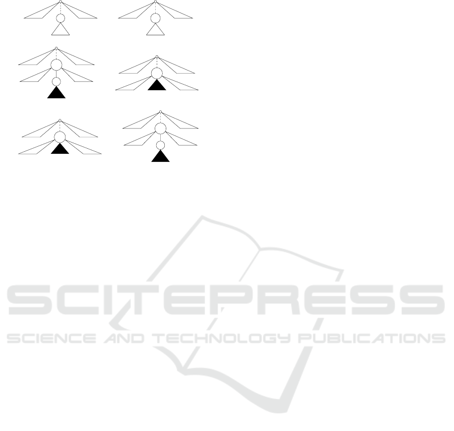
Proof. Consider T

and T

illustrated in Figure 2. It

is obvious that |T

| = |T

| = 2n+ 1. Also it holds that

TAI

) = 2 because M

in Figure 2 is the mini-

mum cost mapping for τ

TAI

. Note that τ

ILST

) =

ALN

) = τ

) = 2.

On the other hand, by the deﬁnition of τ

, we

construct the mapping with cost 0 between hc(T

) and

hc(T

), that is, the second child of the root in T

(la-

beled by a) is corresponding to the third child of the

root in T

(labeled by a) and the third child of the

root in T

(labeled by b) is to the second child of the

root in T

(labeled by b). Then, M

in Figure 2 is the

minimum cost mapping for τ

. Hence, it holds that

) = 2n− 4.

n − 1

n − 2

n − 1

n − 2

Figure 2: Trees T

and T

in Lemma 1 and the minimum

cost mappings M

for τ

TAI

and M

for τ

Lemma 2. There exist trees T

and T

such that

| = |T

| = O(n), τ

TAI

) = τ

) = O(1)

but τ

ILST

) = Ω(n).

Proof. Consider T

and T

illustrated in Figure 3. It is

obvious that |T

| = |T

| = 2n+ 1. Since T

and T

are

caterpillars, it holds that τ

TAI

) = τ

) =

) = 1. Note that τ

ALN

) = 1 and

) = 3.

On the other hand, the minimum cost isolated-

subtree mapping maps r

= r(T

) to r

= r(T

), n+ 1

children of r

to n + 1 children of r

, so the number

of the remained (non-mapped) vertices is n− 1 + n =

2n−1. Hence, it holds that τ

ILST

) = 2n−1.

ICPRAM 2020 - 9th International Conference on Pattern Recognition Applications and Methods

202

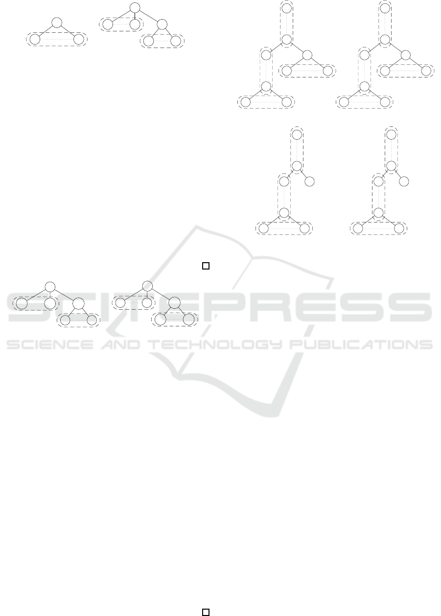
a a

Figure 3: Trees T

and T

in Lemma 2.

Lemma 3. There exist trees T

and T

such that

| = |T

| = O(n), τ

TAI

) = τ

) = O(1)

but τ

ALN

) = Ω(n).

Proof. Consider trees T

and T

in Figure 4. It is

obvious that |T

| = |T

| = 2n + 2. Since T

is trans-

formed to T

by inserting a vertex labeled d in T

af-

ter deleting a vertex labeled by d in T

, it holds that

TAI

) = 2. Since T

and T

are caterpillars, it

also holds that τ

) = τ

) = 2. Note

that τ

) = 4.

On the other hand, the minimum cost alignable

mapping maps a vertex labeled by b (resp., c) in T

to a vertex labeled by c (resp., b) in T

injectively.

Then, it holds that τ

ALN

) = 2n. Also it holds

that τ

ILST

) = 2n.

b d

c c

b b

Figure 4: Trees T

and T

in Lemma 3.

Lemma 4. There exist trees T

and T

such that

| = |T

| = O(n), τ

TAI

) = τ

) = O(1)

but τ

) = Ω(n).

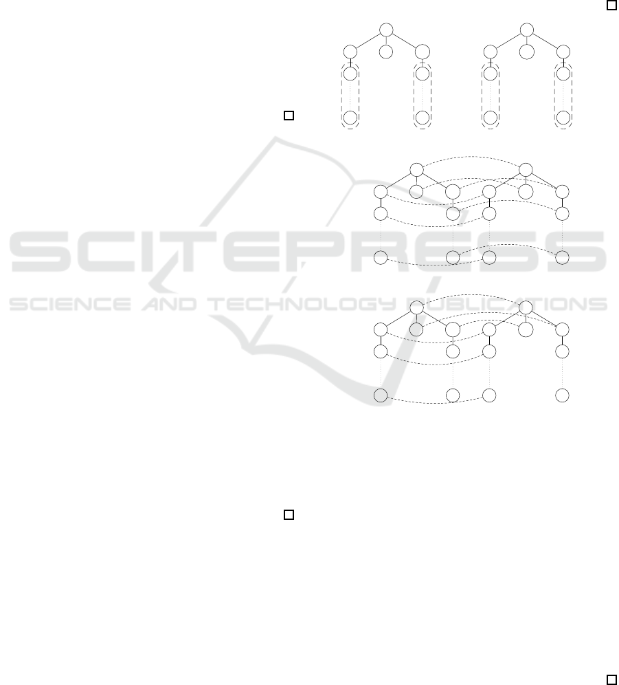
Proof. Consider T

and T

illustrated in Figure 5 (cf.,

(Kan et al., 2014)) and let C

= hc(T

) (i = 1,2). It is

obvious that |T

| = 4n and |T

| = 4n−2. Also it holds

that τ

TAI

) = 2.

For C

and C

in Figure 5, it holds that

) = τ

TAI

) + 2n = 2n + 2. Since the

minimum cost mapping for τ

TAI

) maps the

rightmost vertex v in C

to the rightmost vertex

w in C

, hc(T

) maps the children of v in T

to the children of w in T

injectively. Hence, it

holds that τ

) = τ

TAI

) = 2. Note that

ILST

) = τ

ALN

) = 2.

On the other hand, since the minimum cost seg-

mental mapping maps to the path with n− 1 vertices

and its n children and the vertex and its n children in

, the number of remained (i.e., non-mapped) ver-

tices is n + 1 in T

and n − 1 in T

, so it holds that

) = 2n.

a a

n − 1

a a

n − 1

a a

Figure 5: Trees T

, T

, C

and C

in Lemma 4.

Lemmas 2, 3 and 4 imply the following theorem.

Theorem 7. The distances τ

and τ

are incompa-

rable with the distances τ

ALN

, τ

ILST

and τ

By incorporating Theorem 6 and 7, we can con-

clude that the heavy caterpillar distances τ

and τ

are tractable variations of the edit distance τ

TAI

incom-

parable with the isolated-subtree distance τ

ILST

4 CONCLUSION

In this paper, we have introduced heavy the caterpil-

lar distances τ

and τ

and shown that they pro-

vide the upper bound of the edit distance τ

TAI

, they

are tractable, in particular, quadratic-time computable

under the unit cost function, and incomparable with

other variations of τ

TAI

presented by (Yoshino and Hi-

rata, 2017). Since τ

ILST

is the most general tractable

variation of τ

TAI

(Yoshino and Hirata, 2017), τ

and

are another tractable variations of τ

TAI

incompa-

rable with τ

ILST

Concerned with Lemma 1, it is possible to avoid

this problem to compute the edit distance (the Tai

mapping) between heavy caterpillars by considering

the occurrences of labels in the descendants. It is a fu-

ture work whether or not we can design a new method

to avoid to this problem.

The heavy caterpillar distances τ

and τ

are

deﬁned by M

) and M

) as opera-

Heavy Caterpillar Distances for Rooted Labeled Unordered Trees

203

tional, whereas other variations of τ

TAI

are based on

the declarative deﬁnition of the Tai mapping. Then, it

is a future work whether or not to give the declarative

deﬁnition of τ

and τ

In general, we cannot determine the heavy path

and then the heavy caterpillar uniquely. Then, it is a

future work to design the method to select the heavy

path and the heavy caterpillar uniquely appropriate to

and τ

Finally, after improving that the heavy caterpillar

distances τ

and τ

are determined uniquely, it is

an important future work to give experimental results

to compare τ

and τ

with the isolated-subtree dis-

tance τ

ILST

for real data.

ACKNOWLEDGMENTS

This work is partially supported by Grant-in-Aid

for Scientiﬁc Research 17H00762, 16H02870 and

16H01743 from the Ministry of Education, Culture,

Sports, Science and Technology, Japan. The au-

thors would like to thank anonymous referees of

ICPRAM’20 for valueable comments to revise the

submitted version of this paper.

REFERENCES

Akutsu, T., Fukagawa, D., Halld´orsson, M. M., Takasu, A.,

and Tanaka, K. (2013). Approximation and parame-

terized algorithms for common subtrees and edit dis-

tance between unordered trees. Theoret. Comput. Sci.,

470:10–22.

Demaine, E. D., Mozes, S., Rossman, B., and Weimann, O.

(2009). An optimal decomposition algorithm for tree

edit distance. ACM Trans. Algo., 6.

Deza, M. M. and Deza, E. (2016). Encyclopedia of dis-

tances (4th ed.). Springer.

Gallian, J. A. (2007). A dynamic survey of graph labeling.

Electorn. J. Combin., 14:DS6.

Hirata, K., Yamamoto, Y., and Kuboyama, T. (2011). Im-

proved MAX SNP-hard results for ﬁnding an edit dis-

tance between unordered trees. In Proc. CPM’11

(LNCS 6661), pages 402–415.

Jiang, T., Wang, L., and Zhang, K. (1995). Alignment of

trees – an alternative to tree edit. Theoret. Comput.

Sci., 143:137–148.

Kan, T., Higuchi, S., and Hirata, K. (2014). Segmental

mapping and distance for rooted ordered labeled trees.

Fundam. Inform., 132:1–23.

Kuboyama, T. (2007). Matching and learning in trees. Ph.D

thesis, University of Tokyo.

Lu, C. L., Su, Z.-Y., and Yang, C. Y. (2001). A new mea-

sure of edit distance between labeled trees. In Proc.

COCOON’01 (LNCS 2108), pages 338–348.

Muraka, K., Yoshino, T., and Hirata, K. (2018). Computing

edit distance between rooted labeled caterpillars. In

Proc. FedCSIS’18, pages 245–252.

Muraka, K., Yoshino, T., and Hirata, K. (2019). Vertical

and horizontal distances to approximate edit distance

for rooted labeled caterpillars. In Proc. ICPRAM’19,

pages 590–597.

Sleator, D. D. and Tarjan, R. E. (1983). A data structure for

dynamoic trees. J. Comput. Sys. Sci., 26:362–391.

Tai, K.-C. (1979). The tree-to-tree correction problem. J.

ACM, 26:422–433.

Wang, J. T. L. and Zhang, K. (2001). Finding similar con-

sensus between trees: An algorithm and a distance hi-

erarchy. Pattern Recog., 34:127–137.

Yamamoto, Y., Hirata, K., and Kuboyama, T. (2014).

Tractable and intractable variations of unordered tree

edit distance. Internat. J. Found. Comput. Sci.,

25:307–329.

Yoshino, T. and Hirata, K. (2017). Tai mapping hierarchy

for rooted labeled trees through common subforest.

Theory of Comput. Sys., 60:769–787.

Zhang, K. (1996). A constrained edit distance between un-

ordered labeled trees. Algorithmica, 15:205–222.

Zhang, K. and Jiang, T. (1994). Some MAX SNP-hard re-

sults concerning unordered labeled trees. Inform. Pro-

cess. Lett., 49:249–254.

ICPRAM 2020 - 9th International Conference on Pattern Recognition Applications and Methods

204