
Production Scheduling based on Deep Reinforcement Learning using
Graph Convolutional Neural Network
Takanari Seito and Satoshi Munakata
Hitachi Solutions East Japan, Ltd., Japan
Keywords: Production Scheduling, Deep Reinforcement Learning, Graph Convolutional Neural Network.
Abstract: While meeting frequently changing market needs, manufacturers are faced with the challenge of planning
production schedules that achieve high overall performance of the factory and fulfil the high fill rate constraint
on shop floors. Considerable skill is required to perform the onerous task of formulating a dispatching rule
that achieves both goals simultaneously. To create a useful rule independent of human expertise, deep
reinforcement learning based on deep neural networks (DNN) can be employed. However, conventional
DNNs cannot learn the important features needed for meeting both requirements because they are unable to
process qualitative information included in these schedules, such as the order of operations in each resource
and correspondence between allocated operations and resources. In this paper, we propose a new DNN model
that can extract features from both numeric and nonnumeric information using a graph convolutional neural
network (GCNN). This is done by applying schedules as directed graphs, where numeric and nonnumeric
information are represented as attributes of nodes and directed edges, respectively. The GCNN transforms
both types of information into the feature values by transmitting and convoluting the attributes of each
component on a directed graph. Our investigation shows that the proposed model outperforms the
conventional one.
1 INTRODUCTION
In recent years, consumers’ needs have diversified,
while the life cycles of products have shortened.
Under these conditions, there are two issues in
manufacturing industries for large-item small-volume
production: First, the issues for managers to shorten
the lead time (LT) from material input to product
shipment and strengthen the ability to respond to
short delivery time. Second, the issue for shop floors
to perform efficiently subject to individual constraints
for each product and production line. It is important
for manufacturing industries to construct a production
schedule that satisfies both managers and shop floors.
To make a production schedule, we use a general
dispatching method (Pinedo, 2012), which makes
schedules by successively allocating operations to
resources based on dispatching rules. A dispatching
rule is a criterion for selecting a remaining operation
and a capable resource. Due to the simplicity of the
existing rules, scheduling staff modify them so that a
schedule satisfies both managers and shop floors, e.g.,
by combining multiple rules and/or adding individual
constraints to the rules. However, to construct a good
rule, we need trial and error based on experiences and
expertise of scheduling staff. Therefore, this work can
be a significant burden. Nowadays, due to labor
shortage, especially in Japan, it is difficult to transfer
the expertise to new staff. Thus, to reduce work load,
we need a technology that automatically constructs a
dispatching rule.
For the automatic construction of a dispatching
rule, Riedmiller et al. (1999) applied deep
reinforcement learning (DRL) to production
scheduling. DRL is a machine learning method that
learns a policy that selects an action for each state
through trial and error. In the application of DRL to
production scheduling, we make many schedules by
using the learnt rule at that time and update the rule
to select a good allocation.
In DRL, a dispatching rule is implemented as a
DNN. The DNN receives a state of schedule-making
and computes the probabilistic values for candidates
of allocations. To construct a good schedule that
satisfies both managers and shop floors, it is
necessary for the DNN to extract two types of
information: the factory’s overall performance and
the fill rate constraint. However, the conventional
DNN does not extract the latter, e.g., the resource
766
Seito, T. and Munakata, S.
Production Scheduling based on Deep Reinforcement Learning using Graph Convolutional Neural Network.
DOI: 10.5220/0009095207660772
In Proceedings of the 12th International Conference on Agents and Artificial Intelligence (ICAART 2020) - Volume 2, pages 766-772
ISBN: 978-989-758-395-7; ISSN: 2184-433X
Copyright
c
2022 by SCITEPRESS – Science and Technology Publications, Lda. All rights reserved

each operation is allocated to and the kind of
operations allocated before or after. Therefore, a
conventional DNN cannot be used to make a schedule
that satisfies both managers and shop floors.
In this paper, we propose a new DNN model that
can deal with both types of information. This model
is based on the following two concepts: 1) a schedule
can be represented as a graph structure and 2) a
feature value of each node on the graph can be
extracted by GCN.
The remainder of this paper is structured as
follows. In section 2, we define the problem and
production scheduling. In section 3, we explain the
method of application of DRL to production
scheduling and present the gaps in previous studies.
In section 4, we propose a method to overcome the
issue. In section 5 and 6, we present the experimental
setup and the results. In section 7, we present the
conclusion and future directions of research.
2 PRODUCTION SCHEDULING
In this paper, we deal with a job shop scheduling
problem (JSP) (Pinedo, 2012) that models large-item
small-volume production and add a practical
extension to it. In a practical setting of the
manufacturing industries, there are master data that
define what can be produced and the orders are
selected from the master data accordingly. To follow
this setting, we define master data (mst for short) and
artificially create a problem from it: transaction data
(trn for short).
Master data is given as sets of items [itm
1
, …,
itm
n
] (itm for short) and resources [rsc
1
, …, rsc
m
]
(rsc for short). An item consists of processes [prc
i1
,
…, prc
im
] (prc for short). A process requires
processing time and one capable resource.
Transaction data is given as a set of jobs [job
1
, …,
job
n
]. A job is related to an item and should perform
all processes of the item. We call these processes
operations (opr for short). An operation should be
allocated to a capable resource of a related process
and follow a sequence of the process.
Algorithm 1: Deep Reinforcement Learning.
1. create
training problems
2. for
1,⋯,
:
3. for each training problem:
4. make
schedules by EG with
5. select the best schedule
6. update the DNN with selected schedules
7. ←Δ
3 DEEP REINFORCEMENT
LEARNING
3.1 Application to Scheduling
To generate a dispatching rule automatically,
Riedmiller et al. (1999) proposed an approach using
DRL. DRL applied to production scheduling
generates a dispatching rule through trials and errors
by repeatedly 1) making many schedules using the
learnt rule at that time to obtain better supervised
allocations and 2) updating the rules to select the
supervised allocations.
In DRL, we make a schedule by successively
allocating operations like in a dispatching method,
but it differs from a dispatching method in that we use
a DNN as a dispatching rule. A DNN receives a state
of schedule-making and computes a policy, which is
a set of probabilistic values for candidates of
allocations. We select an allocation from the
candidates that maximize the probabilistic value. A
good schedule can be made by increasing the
probabilistic value of a good allocation.
We show a general DRL algorithm in Algorithm
1. To construct a dispatching rule that makes a good
schedule for several problems, we prepare
training problems from the master data. The
algorithm consists of two phases and repeat it
times.
In the first phase, we make
schedules for
each training problem to obtain better supervised
allocations by using an epsilon-greedy method (EG).
For each scheduling step, we select an allocation by
using the learned DNN or randomly with a
probability 1 or . The search ratio is
initialized to
and updated to Δ at the end of a
training step.
In the second phase, we update the DNN so as to
increase the probabilistic values of supervised
allocations obtained in the previous phase. To reduce
computational time and learn the best allocations, we
select one schedule for each training problem that
maximizes the value of a schedule. For each selected
schedule and each scheduling step, we evaluate an
error between an output of the DNN and a supervised
allocation by a mean-squared error criterion (MSE)
with one-hot representation and minimize them by
Adam (Kingma et al., 2014) with default hyper
parameters. (Although it is better to use a cross-
entropy error criterion for the one-hot representation
in general, we extracted better ability of the DNN in
the MSE.)
Production Scheduling based on Deep Reinforcement Learning using Graph Convolutional Neural Network
767

3.2 Issues in Previous Studies
As mentioned in section 1, planning production
schedules to satisfy the requirements of both factory
management and operations is an urgent problem for
manufacturers. When making schedules,
manufacturers have to simultaneously consider the
factory’s overall performance and the fill rate
constraint on shop floors.
In the DRL framework, we construct a reward
function based on the information to learn a better
policy of allocating operations by repeatedly making
trial production schedules and evaluating them. As
such, it is necessary for a DNN to extract feature
values that include both the information from the trial
schedules satisfactorily. In general, it is easy to create
a DNN model that deals with feature values of the
factory’s overall performance as they are usually
presented as numeric indices such as LT and
availability. On the other hand, conventional DNN
models, which are used in previous studies
(Riedmiller et al., 1999; Zhang et al., 1995; Gabel et
al., 2008), cannot extract feature values characterized
by the satisfaction of the fill rate constraint. This is
because such feature values are comprised of
nonnumeric information about the schedules such as
the resource each operation is allocated to and the
kind of operations allocated before or after. It is
difficult for a DNN model to accept the
abovementioned nonnumeric information as input
and transform them into feature values.
For example, Riedmiller et al. (1999) used only
numeric information to extract feature values of
schedules, e.g., tightness of a job with respect to its
due date, an estimated tardiness, and an average slack.
Thus, it is very hard to address the issues of
production scheduling by employing the previous
methods, which cannot deal with feature values of
nonnumeric information in trial schedules. Therefore,
we have to overcome this limitation of the
conventional DNN model to learn a better policy of
allocating operations for manufacturers so that
production schedules contribute towards both
satisfactory factory performance and higher fill rate
constraint.
4 PROPOSED METHOD
To recognize both numeric and nonnumeric
information by a DNN, we propose a new DNN
model. Our approach is based on two concepts: 1) a
schedule can be represented as a graph structure, 2) a
feature value of each node on the graph can be
extracted by GCN. In the graph structure of a
schedule, we can represent numeric information as
attribute values on nodes, and nonnumeric
information as edges. In the GCNN, we can extract
feature values on nodes from its adjacent relations
defined by edges through graph convolutional
operations. Therefore, we can extract feature values
of nodes with respect to both numeric and
nonnumeric information.
In section 4.1 and 4.2, we elaborate on the two
basic concepts, respectively. In section 4.3, we add an
enhancement that reduces the computational time of
the proposed DNN. In section 4.4, we explain how to
make a schedule by using the proposed DNN.
4.1 Schedule Graph
A graph structure is a data structure that consists of
sets of nodes and edges. The relation of two nodes can
be represented by an edge in a graph structure.
In a schedule graph, a node is used to represent a
component of a schedule as shown in Table 1. A
“block” column is used in section 4.3. We divide the
node type of operation into “allocated operation” and
“unallocated operation” so that a DNN can recognize
the difference between the two.
Numeric information is represented as attribute
values on nodes, e.g., an ability on rsc, processing
time on prc, and working period on a/uopr. An ability
attribute on the resource node is used to represent a
difference among resources with the same function.
For unallocated operations, we use the earliest start
and end time that can be allocated because we cannot
use a determined value.
Nonnumeric information is represented as
directed edges, as shown in Table 2, e.g., process
sequence (process) is from/to prc, capable resource of
a process is an edge from prc to rsc, and allocated
resource of an operation is an edge from aopr to rsc.
There are redundant edges as well: process
sequence edge (operation) and capable resource edge
(operation). They are not necessary for defining the
state of a schedule because using a process sequence
edge (process) and a capable resource edge (process)
is sufficient. As such, we use them to improve the
efficiency of a GCN by connecting nodes that are not
connected with a minimum element.
We show an example of a schedule graph in
Figure 1. The graph on the right represents the state
of a schedule, which is depicted on the left. Rsc (X,
Y, and Z), prc (A ~ G), aopr (1, 2, 4, and 6), and uopr
(3, 5 and 7) are defined as nodes. For simplicity, we
do not show a capable resource edge (operation). For
example, process sequence edge from prc A to prc B
ICAART 2020 - 12th International Conference on Agents and Artificial Intelligence
768
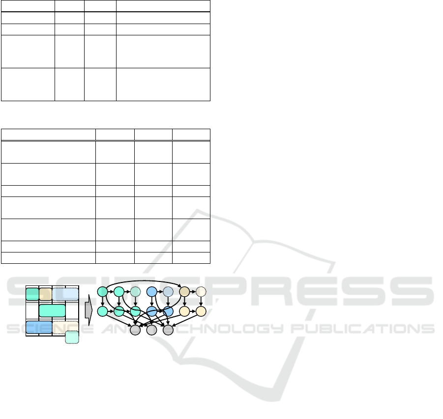
Table 1: Node types of schedule graph.
Name Short Block Attributes
Resource rsc mst Ability
Process prc mst Processing time
Unallocated
Operation
uopr trn
Start date and time,
End date and time,
Working time
Allocated
Operation
aopr sch
Start date and time,
End date and time,
Working time
Table 2: Directed edge types of schedule graph.
Name Block From To
Process sequence
(Process)
mst prc prc
Capable resource
(Process)
mst prc rsc
Operation process trn/sch u/aopr prc
Process sequence
(Operation)
trn/sch u/aopr u/aopr
Capable resource
(Operation)
trn/sch u/aopr rsc
Operation sequence sch aopr aopr
Allocated resource sch aopr rsc
Figure 1: Example of a schedule graph.
implies that prc A is a front process of prc B and prc
B should be performed after prc A; allocated resource
edge from aopr 1 to rsc X implies that aopr 1 is
allocated to rsc X; and operation sequence edge from
aopr 1 to aopr 6 implies that aopr 6 is to be processed
after aopr 1 in the same resource.
This graph needs to be updated when a new
operation is allocated. For example, we assume that
uopr 3 is to be allocated to rsc Z after aopr 4. At first,
node and edge types related to uopr 3 are changed
from uopr to aopr. Next, the following edges are
added to the graph: an operation sequence edge from
aopr 4 to aopr 3 and an allocated resource edge from
aopr 3 to rsc Z.
4.2 Graph Convolution
A GCNN is a form of DNN architecture that is
developed to work on a graph structure (Gilmer et al.,
2017). We define feature values on the nodes of a
GCNN and update them by integrating them with
their adjacent nodes. Through these processes, the
feature values evolve into distinct values that contain
information of their adjacent relations. We can obtain
feature values of schedule components with both
numeric and nonnumeric information and compute a
policy with respect to them in a GCNN applied to a
schedule graph.
Our GCNN consists of three layers: 1) an input
layer, 2) a convolution layer, and 3) an output layer.
All equations are shown from (1) ~ (10) below.
implies concatenation and ⋅ implies inner product.
and imply a number of computations. To recognize
the differences in nodes and edges, we use different
parameters in ,,,,,,GRU,LSTM for each
index ,,,, and in/out types of directed edges. All
parameters are initialized by the Xavier’s method
(Glorot et al., 2010).
1) Input layer
(1)
2) Convolution layer
,
,
,
,
(2)
,
∈
,
(3)
GRU
,⋯,
#
,
(4)
3) Output layer
,
,
,
,
,
(5)
,
,
(6)
⋅
(7)
Softmax
,⋯,
#
(8)
∈
(9)
,
LSTM
,
,
,
(10)
In input layer (1), we initialize a feature value
of node by an affine transformation from an
attribute value
. Although the dimensions of the
attribute values differ from each other, the
dimensions of the feature values are unified to .
In a convolution layer, we integrate adjacent
relations to a feature value. This layer consists of two
functions: 2-1) a message function and 2-2) an update
function. In a message function, for node and its
X
Y
Z
1
2
6
4
7
3
5
time
0
1
2
3
4
X Y Z
A B C D E F G
1 2 3 4 5 6 7
Production Scheduling based on Deep Reinforcement Learning using Graph Convolutional Neural Network
769

adjacent node connected by edge type , we compute
a message
,
from node to node through edge
type in (2) and aggregate the messages that are
categorized in the same edge type to one message
in (3). Adj
,
denotes a set of adjacent nodes
to node connected by edge type . In update function
(4), we reflect aggregated messages
on a
feature value
of node using a gated recurrent unit
GRU
(Cho et al., 2014). #edge denotes the number of
edge types that are connected to node .
Nonnumeric information, represented as adjacent
relations, is transformed to computations such that
each node receives messages from its adjacent nodes
only. Moreover, by repeating this layer
times, the
entire information of the graph is reflected through
feature values because feature values of indirectly
connected nodes are propagated to each node.
We compute a policy in an output layer from
feature values computed in a convolution layer. At first,
we compute a feature value of a candidate of an
allocation in (5). We use several feature values to
represent a candidate with rich information: uopr to
be allocated, rsc where uopr is to be allocated, aopr
and that are processed before/after uopr .
Next, we compute a policy from a set of feature
values of candidates by Set2Set architecture (Vinyals
et al., 2015) in (6)-(10). Set2Set architecture is
designed to work on a set of vectors and computes a
feature value of the set itself. We compute a weight
for each candidate of the set in (7) and (8) and
summarize them in (9) as a feature value
of the set.
#cnd and Cnd denotes a number and a set of
candidates, respectively. A feature value
is used to
update hidden values
,
of candidate by a long
short-term memory LSTM
,
(Hochreiter et al., 1997)
in (10). By repeating (7)-(10)
times, complete
information of all candidates are reflected on feature
value
and weight
. In this paper, we use the
weight
as a policy.
As mentioned above, by using integrated feature
values of both complete and detailed information, we
can compute a policy with respect to the requirements
of both managers and shop floors.
4.3 Speed-up of GCNN Computation
In the original concept of a GCNN in section 4.2, we
re-make the feature values of all the nodes and
convolute them using all the edges every time when
selecting an allocation. However, there are minute
changes between a schedule graph and its updated
version, e.g., an operation sequence edge from aopr 4
to aopr 3 and an allocated resource edge from aopr 3 to
rsc Z in the example in section 4.1. Assuming that there
are few differences in the feature values of nodes with
no change, almost all nodes have only a few
differences in their feature values.
Therefore, to reduce computational time, we re-use
feature values computed in previous scheduling steps
and update them for nodes with changes only: dopr 2,
3, 4, prc C, and rsc Z in the example of section 4.1. We
call this partial convolution. To construct a partial
convolution, we reference a GCNN that can deal with
a dynamic change in graph structure (Manessi et al.,
2020; Ma et al., 2018).
An overview of a GCNN with partial convolution
is shown in Figure 2. We prepare three blocks of
GCNNs: 1) a master block, 2) a transaction block, and
3) a scheduling block, by combining layers of the
original GCN. A scheduling block has a main function
that updates feature values on nodes with changes only
and is executed every time when selecting an allocation.
We use the master and transaction blocks to extract
feature values before we start scheduling.
Figure 2: Overview of graph convolutional neural networks
with partially convolution.
Algorithm 2: Scheduling with partial convolution.
1. execute master block
2. execute transaction block
3. initialize schedule
4. while schedule is not completed:
5. compute a policy by output layer
6. select an allocation by EG or top-k
7. update the schedule
8. execute scheduling block
9. return schedule
We show a procedure of scheduling with partial
convolution in Algorithm 2. At first, we initialize
feature values of nodes categorized to a master block
by an input layer and convolute
times with nodes
and edges categorized under a master block by a
convolution layer. Then, we initialize feature values on
nodes categorized under transaction block by an input
layer and convolute
times with nodes and edges
categorized under both master and transaction blocks.
Thereafter, we can start scheduling. When we select an
allocation, we compute a policy by an output layer with
the feature values at that time. After an operation is
mst
trn/sch
input conv
input
conv
output conv
1) master block
2) transaction bloc
k
3) scheduling block
ICAART 2020 - 12th International Conference on Agents and Artificial Intelligence
770
allocated, we update feature values of nodes with the
changes by a scheduling block
times.
4.4 How to Make a Schedule with DNN
Our DNN acquired a rich representation power and it
can memorize a lot of supervised allocations.
However, it is hard for the DNN to memorize all of
them. There are always some mistakes in allocations
in scheduling with a DNN.
Moreover, we make a schedule by successively
selecting allocations and do not change a previously
decided allocation. Therefore, there is some
possibility that mistakes at the opening step of
scheduling leads to the creation of a bad schedule.
To overcome these mistakes made by the DNN,
we make
schedules as candidates and select one
that maximizes the value of a schedule. When we
make candidates of schedules, we use candidates of
allocations in only top-k of the probabilistic values
and randomly select one from among them.
5 EXPERIMENT
We conduct an experiment to evaluate whether the
value of a schedule made by the proposed method for
problems not used in training gets better with the
number of times of training.
We use a benchmark problem swv11 (50 items
and 10 resources) in OR-Library (Beasley, 1990-
2018). The abilities of resources are unified to 1.0. To
create an artificial problem, we pick up 50 items
randomly from the master data by allowing
duplication. Therefore, each problem has 500
operations.
We evaluate a completed schedule by a makespan
that is related to shortening LT from the perspective
of managers and a degree of satisfaction of basic
constraints of JSP from the perspective of shop floors.
A makespan is a time span from start time to end time
in which all operations are performed. In this paper,
to simplify the problem, we assume that all candidates
of allocations satisfy the basic constraints.
We compare the proposed method (conv.) with
the one without convolution (no conv.). The
comparison uses only numeric information (attribute
values) and leaves out nonnumeric information
(adjacent relations). This enables us to evaluate
whether we need to use nonnumeric information to
construct a good dispatching rule. Moreover, we use
a dispatching method that is used for large-scale
problems. A dispatching rule is the earliest start time
rule as this rule makes the best schedule in a
preliminary experiment.
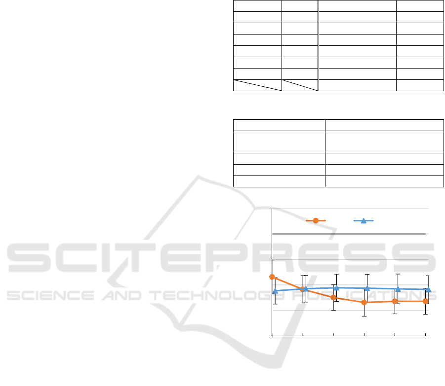
Table 3: Setups of hyper parameters.
128
5
128
16 / 0
128
16 / 0
128
1 / 0
1.0
8
Δ
0.1
8
top-k 2 Epoch 500
Mini-batch 4,000
Table 4: Experimental conditions.
OS Windows 10 Pro
CPU
Intel Core i7-6700HQ,
2.60 GHz
Memory size 16.0 GB
Core number 8
DNN framework PyTorch (1.0.1)
Figure 3: Result of experiment.
The procedure of the experiment is as follows.
First, we prepare
test problems. Next, we train a
DNN with the algorithm 1 with the training problems.
After step 6, we make a schedule for each test
problem using the method in section 4.4 and evaluate
their makespan. The setups of hyper parameters and
experimental conditions are shown in Table 3 and
Table 4, respectively.
6 RESULT
The results of the experiment are depicted in Figure 3.
We use the ratio of makespan to dispatching method as
0.8
0.85
0.9
0.95
1
1.05
012345
Ratio to dispatching method
Training number of time
conv. no conv.
Production Scheduling based on Deep Reinforcement Learning using Graph Convolutional Neural Network
771

each problem has a different makespan. The mean
values and standard deviations of
schedules are
presented in the figure 3. It takes about five weeks for
complete training and about 100 seconds to make
candidates of schedules.
The values derived by the proposed method
with/without convolution are better than a dispatching
method, even without training (number of times of
training is 0). Thus, it is likely that they find a good
schedule by making a lot of candidates, which is not an
effect of convolutions.
A result worth noting is that a value given by the
proposed method with convolutions improves with the
number of times of training and outperforms the one
without convolutions, which do not give the same
results. With number of times of training at
, we
achieve an 87 %, 95 %, or 97 % reduction in makespan
as compared to a dispatching method, where number
of times of training is 0, and the proposed method
without convolution. These differences are significant
as per the t-test, which gives 0.05. Therefore, we
consider that the proposed method can select an
appropriate allocation for each state of schedule-
making because the DNN can recognize the state of
making the schedule in detail as a result of
convolutions.
7 CONCLUSION
We study the DRL method for learning dispatching
rules automatically. Our contribution to the existing
literature is a new DNN model that can recognize both
numeric and nonnumeric information of schedule-
making by applying graph structure of a schedule and
a GCNN. Moreover, we reduce computational time of
the GCNN by applying a partial convolution. After
training a DNN using the DRL algorithm, we observed
that the value of a schedule made by the proposed
method for problems not used in training improves
with the number of times of training. Therefore, we can
automatically construct a good dispatching rule and
expect to reduce the work load for scheduling staff.
However, this paper shows that the proposed
method works on a restricted setting only. To use this
method in a practical scenario, additional experiments
and enhancements need to be conducted. First, the
proposed method should work on problems with a
scale of 1,000 operations. Second, the proposed
method should make a schedule subject to individual
constraints.
ACKNOWLEDGEMENTS
We would like to thank Editage (www.editage.com)
for English language editing.
REFERENCES
Beasley, J. E. (1990-2018). Job shop scheduling problem
swv11 (Online), OR-Library, November 7, 2019,
http://people.brunel.ac.uk/~mastjjb/jeb/info.html
Cho, K., Van Merriënboer, B., Gulcehre, C., Bahdanau, D.,
Bougares, F., Schwenk, H., & Bengio, Y. (2014).
Learning phrase representations using RNN encoder-
decoder for statistical machine translation. arXiv
preprint. arXiv:1406.1078.
Gabel, T., & Riedmiller, M. (2008). Adaptive reactive job-
shop scheduling with reinforcement learning agents.
International Journal of Information Technology and
Intelligent Computing, 24.
Gilmer, J., Schoenholz, S. S., Riley, P. F., Vinyals, O., &
Dahl, G. E. (2017). Neural message passing for quantum
chemistry. Proceedings of the 34th International
Conference on Machine Learning, (Vol. 70) (pp. 1263–
1272).
Glorot, X., & Bengio, Y. (2010). Understanding the difficulty
of training deep feedforward neural networks.
Proceedings of the 13th International Conference on
Artificial Intelligence and Statistics (pp. 249–256).
Hochreiter, S., & Schmidhuber, J. (1997). Long short-term
memory. Neural Computation, 9, 1735–1780.
Kingma, D. P., & Ba, J. (2014). Adam: A method for
stochastic optimization. arXiv preprint. arXiv:1412.
6980.
Ma, Y., Guo, Z., Ren, Z., Zhao, E., Tang, J., & Yin, D. (2018).
Streaming graph neural networks. arXiv preprint
arXiv:1810.10627.
Manessi, F, Rozza, A., & Manzo, M. (2020). Dynamic graph
convolutional networks. Pattern Recognition, 97,
107000.
Pinedo, M. L. (2012). Scheduling: Theory, Algorithms, and
Systems (4th ed.). New York: Springer.
Riedmiller, S., & Riedmiller, M. (1999). A neural
reinforcement learning approach to learn local
dispatching policies in production scheduling.
Proceedings of the 16th International Joint Conference
on Artificial Intelligence (Vol. 2) (pp. 764–469).
Vinyals, O., Bengio, S., & Kudlur, M. (2015). Order matters:
Sequence to sequence for sets. arXiv preprint.
arXiv:1511.06391.
Zhang, W., & Dietterich, T. G. (1995). A reinforcement
learning approach to job-shop scheduling. International
Joint Conferences on Artificial Intelligence (Vol. 95) (pp.
1114–1120).
ICAART 2020 - 12th International Conference on Agents and Artificial Intelligence
772
