A Manifold Learning Framework for the Detection of Cardiac Disorders

in Acoustic Signals

Keren Hochman

, Amir Averbuch

, Alon Schclar

and Raid Saabni

School of Computer Science, Tel Aviv University, POB 39040, Tel Aviv 69978, Israel

School of Computer Science, The Academic College of Tel-Aviv Yaffo, POB 8401, Tel Aviv 61083, Israel

Keywords:

Cardiac Disorder Detection, Manifold learning, Dimensionality Reduction, Acoustic Signal.

Abstract:

Cardiac disorders are clinical situations in which the heart does not function properly. These disorders may

be fatal to patients if they are not detected. Detecting such disorders often involves special and in some cases

very expensive medical devices such as Computer Tomography (CT), Magnetic Resonance Imaging (MRI),

Ultrasound imaging or Electrocardiograms. Acoustic detection of these disorders by simply listening to the

heart using a stethoscope - although being the cheapest detection method - requires a highly skilled doctor. We

propose a method that detects cardiac disorders from simple acoustic recordings of the heart. Acquiring such

recording is in most cases cheaper than the above mentioned devices. The proposed algorithm is composed

of two steps: an ofﬂine training step which constructs a classiﬁer based on labeled recordings; and an online

classiﬁcation step which detects cardiac disorders given a recording of the heart. Given the online nature

of the algorithm, the proposed algorithm can be implemented as a smartphone application. One of the key

elements of oth the training and detection steps is the concise and informative representation of the acoustic

signal. This representation is obtained using the application of the spline wavelet packet transform followed

by the application of the Diffusion Maps (DM) dimensionality reduction algorithm. The proposed approach is

generic and can be applied to various signal types for solving different classiﬁcation problems.

1 INTRODUCTION

Classiﬁcation of acoustic signals is a contemporary

problem whose application is found in many domains

e.g. Biology (Mac et al., 2018), Surveillance (Mu-

nich, 2004; Yaan Li and Zhe Chen, 2017; Schclar

et al., 2010; Averbuch et al., 2001; Averbuch et al.,

2004) and oceanic sciences (D.A.Abraham, 2019),

to name a few. In this paper we focus on detec-

tion of cardiac disorders using acoustic recordings of

the heart. The underlying assumption is that record-

ings of cardiac disorders have distinctive acoustic sig-

natures which differ from the acoustic signatures of

healthy hearts. In order to detect cardiac disorders us-

ing acoustic recordings, one must extract and recog-

nize these deﬁnitive signatures. These signatures can

be found in small intervals in the recording. There-

fore, we decompose the signal into short overlapping

windows that are used by the proposed algorithm.

Each window is treated as a high dimensional data

point.

Using the raw signal is inefﬁcient and produces

poor results since the signal contains redundant in-

formation and noise. The redundant information is

partly due to the quasi-periodic structure of the signal

which contains only a small number of dominant fre-

quencies. Accordingly, we apply the Spline Wavelet

Packet Transform (SWPT) (Daubechies, 1992) to

each window since we assume that acoustic sig-

natures are inherent in the energy of the wavelet

packet coefﬁcients. Furthermore, SWPT sparsiﬁes

the smooth parts of the signal, providing better energy

compactization of the signal in a few wavelet packet

coefﬁcients and provides better frequency coverage of

the signal.

In order to remove noise that is still present after

the application of the SWPT and derive a more con-

cise representation (using the high dimensional result

of the SWPT is impractical due to the curse of dimen-

sionality) we apply the Diffusion Maps (DM) (Coif-

man and Lafon, 2006; Schclar, 2008) dimensionality

reduction algorithm to the result of the SWPT. This

embeds the high dimensional result of the SWPT into

a lower dimension space. We chose the DM algorithm

since it was successfully applied in various algorithms

(Lafon and Lee, 2006; Lafon et al., 2006; Rabin and

Coifman, 2012; Deng and Han, 2016; Sulam et al.,

2017).

In order to derive the concise representation of a

new signal s

new

, we use the Nystr

om out-of-sample

192

Hochman, K., Averbuch, A., Schclar, A. and Saabni, R.

A Manifold Learning Framework for the Detection of Cardiac Disorders in Acoustic Signals.

DOI: 10.5220/0009094401920197

In Proceedings of the 9th International Conference on Pattern Recognition Applications and Methods (ICPRAM 2020), pages 192-197

ISBN: 978-989-758-397-1; ISSN: 2184-4313

extension (Nystr

om, 1928) algorithm instead of ap-

plying the DM algorithm. We do so since the com-

plexity of the Nystr

om algorithm is linear while the

complexity of the DM algorithm is quadratic.

The proposed algorithm is composed of two

stages:

• An ofﬂine training stage in which data with a-

priory knowledge is analyzed and features, which

characterize it, are extracted and stored.

• An online detection phase in which a new signal

that was part of the training stage undergoes pro-

cessing stages that are similar to the training stage.

The processing outcome is compared using a sim-

ple k-nearest neighbor scheme to the database that

was constructed in the training stage.

The rest of the paper is organized as follows. In Sec-

tion 2 we brieﬂy describe the SWPT, DM and the

Nystr

om algorithms. In section 3 the proposed algo-

rithm is presented. Experimental results are presented

in section 4. In section 5 we summarize the results

and outline the next steps in this research.

2 MATHEMATICAL

BACKGROUND

2.1 Spline Wavelet Packets

There are many wavelet packet libraries which dif-

fer from each other by their generating low-pass and

high-pass ﬁlters, the shape of their basic waveforms

and their frequency contents. In principle, the trans-

form of a signal of length n = 2

can be implemented

up to the j

decomposition level (scale). At this

level, there exist n different waveforms, which are

close to sine and cosine waves with multiple frequen-

cies. There is a duality in the nature of the wavelet

packet. As the decomposition level increases, a better

frequency resolution at the expense of time domain

resolution is achieved and vice versa.

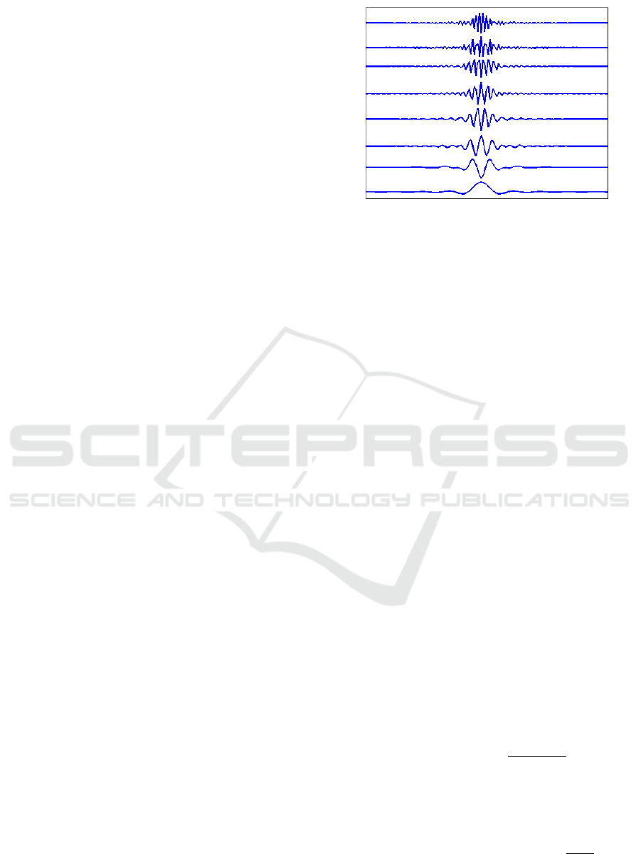
Figure 1 displays a wavelet packet after decompo-

sition into three levels by a spline of sixth order (Bat-

tle -Lemarie (Daubechies, 1992)). The splines do not

have a compact support in the time domain. However,

they produce an excellent splitting of the frequency

domain (see Fig. 1-b).

The advantage of spline wavelet is that it produces

a good split of the frequency domain, however, it is

not localized as well as other wavelet packets. In this

paper we chose the sixth order spline wavelet packets

since it reduces the overlap between frequency bands

associated with different decomposition blocks, while

Figure 1: Spline of the sixth order wavelet packet in the

third scale‘.

providing a variety of waveforms with a fair time do-

main localization.

2.2 The Diffusion Maps Algorithm

Diffusion maps (Coifman and Lafon, 2006; Schclar,

2008), is a nonlinear dimensionality reduction

method. The eigenfunctions of a Markov matrix,

which deﬁne a random walk on the data, are used to

construct coordinates that provide concise representa-

tions of the underlying data sets where the geometry

of the original data set is preserved.

Consider a data set Ω = {x

,...x

}, x

∈ R

, m ∈

N. An undirected weighted graph in which each node

corresponds the a data point is constructed. Every pair

of nodes x

∈ Ω, i 6= j, 1 ≤ i < j ≤ n is connected

by an edge whose weight is given by a symmet-

ric, point-wise non-negative weight function w(x

which reﬂects the similarity between x

and x

. The

DM algorithm embeds Ω into a low-dimensional L

space in which the Euclidean distance between points

i and j approximates the connectivity between these

points in the graph. The connectivity is referred to as

the diffusion distance.

The choice of the weight function is dependents

on the application as long as the conditions of sym-

metry and non-negativity are kept. A common choice

for the kernel function, w(x

), is the Gaussian ker-

nel

w(x

) = exp



−

||x

− x



(1)

where ε > 0 is the scale parameter. Discussion on how

to choose ε can be found in (Schclar and Averbuch,

2015).

We now create a random walk on the data set

Ω by forming the kernel p(x,y) =

w(x,y)

d(x)

where

d(x) =

∑

z∈Ω

w(x,z) is the degree of x. Since p(x,y) ≥

0 and

∑

y∈Ω

p(x,y) = 1, this deﬁnes a Markov chain

A Manifold Learning Framework for the Detection of Cardiac Disorders in Acoustic Signals

193

where p(x, y) is the probability to jump from x to y

in a single step. Let P be the N × N transition ma-

trix of this Markov chain. Let p

(x,y) be the ker-

nel corresponding to the t

power of matrix P, that

is, p

(x,y) is the transition probability matrix in t

time steps. When t →+∞, this Markov chain is gov-

erned by a unique stationary distribution φ

, such that

lim

t→∞

(x,y) = φ

(y) for all x and y. φ

is the top

left eigenvector of P, φ

P = φ

, and φ

(y) =

d(y)

∑

∈Ω

d(z)

holds. Let {φ

} and {ψ

} be the corresponding bi-

orthogonal left and right eigenvectors of P. The fol-

lowing eigendecomposition exists

(x,y) =

n−1

∑

l=0

(x)φ

(y) (2)

where {λ

} is the sequence of eigenvalues of P (with

|λ

| ≥ |λ

|...).The diffusion distance between two

points x and z was introduced in (Coifman and Lafon,

2006) as

(x,z) =

∑

y∈Ω

((p

(x,y) − (p

(z,y))

(y)

. (3)

This distance measures the connectivity between x

and z since it involves an integration along all paths

of length t starting from x or z. Unlike the shortest

path or geodesic distance, this metric is robust to noise

(perturbation) due to this integration.

The connection between the diffusion distance

and the eigenvectors is given by

(x,z) =

∑

l≥1

(ψ

(x) − ψ

(z))

. (4)

Note that ψ

does not appear in the sum because it is

a constant.

Due to the spectrum decay, only a few number of

terms are needed to achieve a given relative accuracy

δ > 0. The number of needed terms is denoted by

m(t). From Eq. 4 it follows that the right eigenvector

can be used to compute the diffusion distance and thus

the diffusion map is deﬁned as

: x → (λ

(x),λ

(x)...,λ

m(t)

(x))

. (5)

This mapping provides coordinates for the data set

Ω and embeds the n data points into the Euclidean

space R

m(t)

. The dimensionality is reduced due to the

fast decay of {λ

} that ensures that m(t) << m.

2.2.1 The Nystr

om Out-of-sample Extension

The Nystr

om extension (NE) (Nystr

om, 1928;

Williams and Seeger, 2000; Fowlkes et al., 2004) ex-

tends a known function on a given data set to include

a new data point which is not int the date set. The

NE algorithm uses both the target function and the

geometry of the training set. We use NE to embed

a new signal into the low-dimensional representation

of the training set. The Nystr

om extension has been

successfully used numerous problems in the past e.g.

to accelerate kernel machines (Williams and Seeger,

2000) and spectral clustering (Fowlkes et al., 2004),

to name a few.

Let Ω be a data set and let Ψ

be its diffusion em-

bedding map. µ

and φ

are the eigenvalues and eigen-

vectors, respectively, of the Gaussian kernel with

width σ on the training data Ω. Denote by Ω the new

data set. σ > 0 deﬁnes the scale of the extension.

Then, µ

(x) =

∑

y∈Ω

−||x−y||

/σ

(y), x ∈ Ω.

Since the kernel can be evaluated in the entire space,

it is possible to use any x ∈ R

on the right side of the

identity.

The Nystr

om extension (Nystr

om, 1928) from

Ωto R

of the eigenfunctions is deﬁned as:

(x) =

∑

y∈Ω

−||x−y||

/σ

(y), x ∈ R

. (6)

Any function on the training set can be decom-

posed into

f (x) =

∑

, f

(x), x ∈ Ω. (7)

The Nystr

om extension of f on the rest of R

given by

f (x) =

∑

, f

(x), x ∈ R

. (8)

In particular, f can be every coordinate in the embed-

ding that the DM algorithm produces.

3 THE PROPOSED ALGORITHM

The classiﬁcation algorithms for processing acoustic

signals is split into two stages, training and detection.

The input to the training stage is a data set Ω =

}

i=1

that is composed of recordings signals in

a pulse mode modulation (PCM) format of healthy

hearts and hearts that suffer from disorders. The

signals may vary in their length and their class/type

are known a-priory. The training stage constructs a

concise representation of the training signals. This

is achieved by embedding the signals into a low-

dimensional space. The detection phase embeds new

signals into the low-dimensional space that was con-

structed during the training phase. A new signal

is classiﬁed into health/unhealthy heart via a simple

nearest neighbor scheme.

Both stages share common data preparation steps

which are described in Algorithm 1 and are detailed

below.

ICPRAM 2020 - 9th International Conference on Pattern Recognition Applications and Methods

194

Algorithm 1: Preprocessing of a signal s.

1. Decomposition of the signal s into overlapping

windows.

2. Application of the spline wavelet packet trans-

form to each window.

3. Summing the wavelet coefﬁcients in each fre-

quency band.

4. Averaging every µ consecutive windows obtained

in step 2 in order to reduce the noise where µ > 0

is a parameter that indicates the number of win-

dows to average.

5. Dimensionality reduction of each averaged win-

dow using DM during training and using the

Nystr

om extension during testing.

The stages differ in a ﬁnal preprocessing stage that

they apply following Algorithm 1. Namely, the train-

ing stage uses the DM algorithm while the detection

phase uses the Nystr

om extension.

Below is a detailed description of each step in Al-

gorithm 1.

Step 1: Decomposition into Windows. Let s

∈ Ω,

be a signal and let s

(t), t = 0,..., |s

| − 1 denote the

modulation value at time t where |s

| is the size of sig-

nal s

. Each signal s

is decomposed into a set of win-

dows W

- each of size l = 2

, r,l ∈ N, with overlap-

ping of ν% between every two consecutive windows.

The set of all windows is given by Ω

= ∪

i=1

}

j=1

, w

∈ R

where n

is the total number of win-

dows of the signals in Ω.

Step 2: Application of the Spline Wavelet Pack-

ets. We use the sixth order spline wavelet packet.

A spline wavelet is applied to scale D ∈ N to each

window w

∈ Ω

. Typically, if l = 2

= 1024, then

D = 6 and if l = 2

= 512 then D = 5. The coef-

ﬁcients are taken from the last scale D. This scale

contains l = 2

coefﬁcients that are arranged into 2

blocks of length 2

r−D

. Each block is associated with

a certain frequency band. These bands form a near

uniform partition of the Nyquist frequency domain

into 2

parts. The outcome is Ω

wave

= {wp

}

j=1

where wp

∈ R

. At the end of this step, each win-

dow wp

∈ Ω

wave

is substituted for the set of its spline

wavelet coefﬁcients.

Step 3: Calculation of the Energy. We construct

the acoustic signature using the distribution of en-

ergy among blocks which consist of wavelet packet

coefﬁcients. The energy is calculated by summing

the coefﬁcients in each block. The outcome is Ω





j=1

where each we

∈ Ω

is of dimension R

This operation reduces the dimension by a factor of

r−D

Step 4: Averaging. This step is applied in order

to reduce perturbations and noise. Given the energy,

Ω

= {we

}

j=1

, of the signals as calculated in step 3,

we calculate the average of every µ consecutive win-

dows which belong to the same signal in order to re-

ceive a more robust signature. Given a training signal

s, let Ω

(s) =



(s)



(s)

j=1

be the set of segments

of wavelet energy coefﬁcients that were calculated in

step 3 for s where n

(s) is the number of segments

that s was decomposed to in step 1. For each segment

(s) we calculate

(s) =

j−µ+1

∑

k= j

(s)

The classiﬁcation of wa

(s) is the same as s. The out-

put of this step is Ω





j=1

, wa

∈ R

Step 5: Dimensionality Reduction. The dimen-

sionality of each segment in the output of step 4 if

further reduced by applying dimensionality reduction.

However, the training and detection stages implement

this step differently. The training stage applies the

DM algorithm to Ω

and produces

Ω





j=1

∈ R

where q is the reduced dimension. The de-

tection step, on the other hand, employs the Nystr

extension algorithm in the following manner.

Let α be a test signal that is input to the detection

stage. In order to classify the k-th segment, α

, where

k ≥ µ, the, steps 1-4 are applied to α

. We denote the

averaged energy of the µ windows that precede α

(note that there is no need to wait for the entire

signal to be received). The Nystr

om extension algo-

rithm is applied to

and we denote the result by

This embeds it into the reduced space that contains

Ω

. The classiﬁcation of

is determined according

to the type of training window that is the nearest to

The classiﬁcation phase is done online. In order to

classify a signal at time t, the algorithm only needs the

µ consecutive overlapping windows that immediately

precede time t.

4 EXPERIMENTAL RESULTS

We denote the parameters of the algorithms by: L is

the window size, ν is the overlapping percent, µ is the

number of windows to average, D is the the scale of

A Manifold Learning Framework for the Detection of Cardiac Disorders in Acoustic Signals

195

spline wavelet and q is the the target dimensionality

of the DM algorithm. The number of neighbors in

the k-nn classiﬁer was set to 15. The values of these

parameters were determined empirically. The classi-

ﬁcation phase was tested on recordings that were not

a part of the training set.

The signals were taken from different people in

different occasions. The recording sample rates (SR)

were 22050 samples per second (SPS) and 11025

SPS. They were all down-sampled to 2205 SPS. The

classes in this experiment are: (a) normal heart beats;

and (b) a cardio vascular disorder. The data were

collected from different adults in different occasions.

The training sample set consisted from 7 recordings,

4 of them represent normal cardio behavior and 3

represent a cardio disorder. The detection set con-

tains 2 recordings that did not participate in the train-

ing phase. The following parameters were used in

the training and classiﬁcation phases: L = 1024, ν =

75%, µ = 3, D = 6, q = 3. These parameters were

determined empirically.

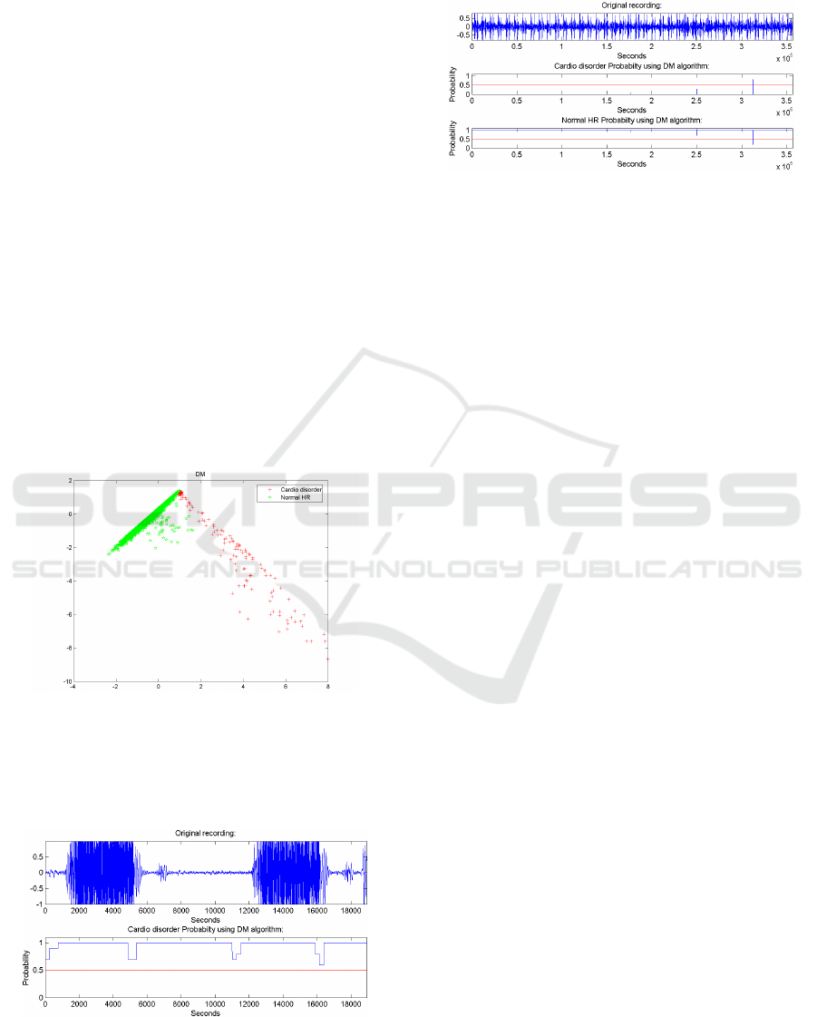
Figure 2 depicts the clusters that are obtained

when the dimension reduced space is R

. It can be

seen that the ﬁrst two eigenvectors provide a complete

separation into two disjoint clusters.

Figure 2: Clusters generated by the application of DM. The

plot is the embedded data onto the space spanned by the ﬁrst

two eigenvectors.

Figure 3 contains the classiﬁcation results of a

recording that contains a cardiac disorder.

Figure 3: Classiﬁcation from a recording that contains a

cardiac disorder. Top: Original recording. Bottom: The

probability for a cardio disorder using the DM algorithm.

Figure 4 contains the classiﬁcation results of a

normal heart beat signal.

Figure 4: Classiﬁcation from a recording that contains a

normal cardio system. Top: Original recording. Middle:

The probability for a cardio disorder using the DM algo-

rithm. Bottom: The probability for a normal cardio behav-

ior using the DM algorithm.

It can be seen that classiﬁcation results are very

good.

5 CONCLUSIONS

In this work, we presented a manifold learning

scheme for the detection of cardiac disorders using

acoustic recordings. The algorithm is composed of a

training phase and a detection phase. In both phases

the signals are decomposed to overlapping windows

and each window undergoes a spline wavelet packet

transform followed by coefﬁcients compaction and

temporal smoothing. The dimensionality of each win-

dow is further reduced via the DM dimensionality re-

duction algorithm. The set of all windows form a

training set for a nearest-neighbor classiﬁer. During

the detection, the examined signal undergoes simi-

lar steps to those employed during the training, how-

ever, the dimension is reduced via the NE algorithm.

Each classiﬁcation of each window in the examined

signal is determined according to its nearest in the

dimension-reduced training set.

The preliminary results of the proposed scheme

are very promising. However, the scheme is further

investigate in as follows. Additional experiments are

needed to corroborate the accuracy of the scheme.

A data-driven method to automatically determine the

optimal values of the algorithm’s parameters is sought

after. Other classiﬁers and other manifold learning al-

gorithms should be examined. The proposed scheme

is general and can be successfully applied to other do-

mains. Finally, the training set can be online extended

to include the new signals.

ICPRAM 2020 - 9th International Conference on Pattern Recognition Applications and Methods

196

REFERENCES

Averbuch, A., Hulata, E., and Zheludev, V. (2004). Identiﬁ-

cation of acoustic signatures for vehicles via reduction

of dimensionality. International Journal of Wavelets,

Multiresolution and Information Processing, 2(1).

Averbuch, A., Hulata, E., Zheludev, V., and Kozlov, I.

(2001). A wavelet packet algorithm for classiﬁcation

and detection of moving vehicles. Multidimensional

Systems and Signal Processing, 12(1).

Coifman, R. R. and Lafon, S. (2006). Diffusion maps. Ap-

plied and Computational Harmonic Analysis: special

issue on Diffusion Maps and Wavelets, 21:5–30.

D.A.Abraham (2019). Underwater Acoustic Signal Pro-

cessing: Modeling, Detection, and Estimation (Mod-

ern Acoustics and Signal Processing). Springer.

Daubechies, I. (1992). Ten Lectures on Wavelets. Society

for Industrial and Applied Mathematics, Philadelphia,

PA, USA.

Deng, S.-W. and Han, J.-Q. (2016). Towards heart sound

classiﬁcation without segmentation via autocorrela-

tion feature and diffusion maps. Future Generation

Computer Systems, 60:13 – 21.

Fowlkes, C., Belongie, S., Chung, F., and Malik, J. (2004).

Spectral grouping using the nystrom method. IEEE

Transactions on Pattern Analysis and Machine Intel-

ligence, 26(2):214–225.

Lafon, S., Keller, Y., and Coifman, R. R. (2006). Data fu-

sion and multicue data matching by diffusion maps.

IEEE Transactions on Pattern Analyss and Machine

Intelligence, 28:1784–1797.

Lafon, S. and Lee, A. (2006). Diffusion maps and coarse-

graining: A uniﬁed framework for dimensionality re-

duction, graph partitioning, and data set parameteri-

zation. IEEE Transactions on Pattern Analysis and

Machine Intelligence, 28(9):1393–1403.

Mac, A. O., Gibb, R., Barlow, K. E., Browning, E., Fir-

man, M., and Freeman, R. (2018). Bat detective - deep

learning tools for bat acoustic signal detection. PLoS

Computational Biology, 14(3).

Munich, M. E. (2004). Bayesian subspace methods for

acoustic signature recognition of vehicles. 12th Eu-

ropean Signal Processing Conference, pages 2107–

2110.

Nystr

om, E. J. (1928).

Uber die praktische auﬂ

osung

von linearen integralgleichungen mit anwendungen

auf randwertaufgaben der potentialtheorie. Commen-

tationes Physico-Mathematicae, 4(15):1–52.

Rabin, N. and Coifman, R. R. (2012). Heterogeneous

datasets representation and learning using diffusion

maps and laplacian pyramids. In Proceedings of the

2012 SIAM International Conference on Data Mining,

pages 189–199.

Schclar, A. (2008). A Diffusion Framework for Dimension-

ality Reduction, pages 315–325. Springer US, Boston,

MA.

Schclar, A. and Averbuch, A. (2015). Diffusion bases di-

mensionality reduction. In Proceedings of the 7th In-

ternational Joint Conference on Computational Intel-

ligence, IJCCI 2015, Lisbon, Portugal, November 12-

14, 2015., pages 151–156.

Schclar, A., Averbuch, A., Hochman, K., Rabin, N., and

Zheludev, V. (2010). A diffusion framework for de-

tection of moving vehicles. Digital Signal Process-

ing,, 20(1):111–122.

Sulam, J., Romano, Y., and Talmon, R. (2017). Dynami-

cal system classiﬁcation with diffusion embedding for

ecg-based person identiﬁcation. Signal Processing,

130:403 – 411.

Williams, C. K. I. and Seeger, M. (2000). Using the nystr

method to speed up kernel machines. In Proceedings

of the 13th International Conference on Neural Infor-

mation Processing Systems, NIPS’00, pages 661–667,

Cambridge, MA, USA. MIT Press.

Yaan Li and Zhe Chen (2017). Entropy based underwater

acoustic signal detection. In 2017 14th International

Bhurban Conference on Applied Sciences and Tech-

nology (IBCAST), pages 656–660.

A Manifold Learning Framework for the Detection of Cardiac Disorders in Acoustic Signals

197

REFERENCES

Averbuch, A., Hulata, E., and Zheludev, V. (2004). Identifi-