Classiﬁcation of Optical Coherence Tomography using Convolutional

Neural Networks

A. A. Saraiva

2,6 a

, D. B. S. Santos

1 b

, Pimentel Pedro

1 c

, Jose Vigno Moura Sousa

1 d

N. M. Fonseca Ferreira

3,4 e

, J. E. S. Batista Neto

, Salviano Soares

3 f

and Antonio Valente

2,5 g

UESPI - University of State Piaui, Piripiri, Brazil

University of Tr

as-os-Montes and Alto Douro,Vila Real, Portugal

Coimbra Polytechnic, ISEC, Coimbra, Portugal

Knowledge Engineering and Decision-Support Research Center (GECAD) of the Institute of Engineering,

Polytechnic Institute of Porto, Portugal

INESC-TEC Technology and Science, Porto, Portugal

University of S

ao Paulo, S

ao Carlos, Brazil

Keywords:

OCT, CNN, Classiﬁcation, K-fol, Labeled Optical Coherence Tomography.

Abstract:

This article describes a classiﬁcation model of optical coherence tomography images using convolution neural

network. The dataset used was the Labeled Optical Coherence Tomography provided by (Kermany et al.,

2018) with a total of 84495 images, with 4 classes: normal, drusen, diabetic macular edema and choroidal

neovascularization. To evaluate the generalization capacity of the models k-fold cross-validation was used.

The classiﬁcation models were shown to be efﬁcient, and as a result an average accuracy of 94.35% was

obtained.

1 INTRODUCTION

An examination known as optical coherence tomog-

raphy (OCT) has gained ground in the latest comple-

mentary clinical tests for the diagnosis of retinal and

vitreous disease (Preti et al., 2018).

This technology was developed by Fujimoto at the

Massachusetts Institute of Technology, applied in the

ophthalmological diagnosis by Puliaﬁto. The use of

this examination has become fundamental in the diag-

nosis, on evolution and postoperative control of mul-

tiple macular conditions (Dimitrova et al., 2017).

According to (Swanson and Fujimoto, 2017) ap-

proximately 30 million procedures of optical coher-

ence tomography (OCT) images are performed per

year, the analysis and interpretation of these images,

https://orcid.org/0000-0002-3960-697X

https://orcid.org/0000-0003-4018-242X

https://orcid.org/0000-0002-5291-0810

https://orcid.org/0000-0002-5164-360X

https://orcid.org/0000-0002-2204-6339

https://orcid.org/0000-0001-5862-5706

https://orcid.org/0000-0002-5798-1298

consumes a signiﬁcant amount of time. OCT helped

patients prevent or minimize vision loss by detecting

retinal diseases in the early stages of treatment (Swan-

son and Fujimoto, 2017).

According to (Sivaprasad and Moore, 2008), the

growth of new choroidal blood vessels is known as

choroidal neovascularization (CNV). These new ves-

sels come from a rupture in the Bruch membrane that

is located in the subretinal pigment epithelium. Ac-

cording to (Baxter et al., 2013) CNV occurs in about

2 to 3% of cases of posterior uveitis.

Diabetic macular edema (DME) is a complication

of diabetes caused by ﬂuid accumulation in the mac-

ula, or central portion of the eye, that causes the mac-

ula to swell (Wells et al., 2016). The macula is ﬁlled

with cells responsible for direct vision that aid in read-

ing and directing (Wells et al., 2016).

When the macula begins to ﬁll with ﬂuid and

swell, the capacity of these cells is impaired, caus-

ing blurred vision (Bressler et al., 2016). The DME

is diabetic retinopathy, in which the blood vessels of

the eye are damaged, allowing the ﬂuid to escape,

this type of disease can also be diagnosed through the

168

Saraiva, A., Santos, D., Pedro, P., Sousa, J., Ferreira, N., Neto, J., Soares, S. and Valente, A.

Classiﬁcation of Optical Coherence Tomography using Convolutional Neural Networks.

DOI: 10.5220/0009091001680175

In Proceedings of the 13th International Joint Conference on Biomedical Engineering Systems and Technologies (BIOSTEC 2020) - Volume 3: BIOINFORMATICS, pages 168-175

ISBN: 978-989-758-398-8; ISSN: 2184-4305

OCT (Gill et al., 2017).

Drusen are small accumulations of yellow or

white extracellular material that accumulate between

Bruch’s membrane and the retinal pigment epithelium

of the eye, which can be detected by OCT (Gaier

et al., 2017). The presence of small Drusen is normal

with advancing age, and most people over 40 have

some Drusen (Alten et al., 2017). However, the pres-

ence of larger and more numerous Drusen in the mac-

ula is an early sign of age-related macular degenera-

tion (DMRI) (Schlanitz et al., 2017).

In this way, he inspired the design an OCT image

classiﬁer, in order to classify three types of patholo-

gies visible in OCT: CNV, DME, and DRUSEN, in

an automated and fast way. The method chosen and

implemented constitutes in the classiﬁcation of OCT

images of retinas of living patients, from this, to iden-

tify whether or not they have any of the diseases

mentioned above. For the classiﬁcation was used

the dataset Labeled Optical Coherence Tomography

with total 84,495 images provided by (Kermany et al.,

2018).

The classiﬁcation stage consists of two sub-steps,

where the ﬁrst is carried out to the training of a deep

learning known as Convolutional Neural Networks

(CNN), the second sub-step is the validation of the

model, that is, the tests with unknown images by CNN

(Saraiva. et al., 2019b), (Saraiva. et al., 2019a). The

method covered ensures a robust coverage in image

recognition, under certain assumptions that will be

clariﬁed throughout the text.

The paper is divided into 5 sections, in which

section 2 is characterized by the description of the

methodology applied, followed by the validation met-

rics in section 3. The results after the application of

the proposal and the ﬁnal conclusions are presented in

sections 4 and 5, respectively.

The data set is organized into 4 categories: NOR-

MAL, CNV, DME, DRUSEN, totaling 84,495 OCT

images. The OTC images were selected from retro-

spective cohorts of adult patients at the Shiley Eye

Institute of the University of California at San Diego,

the California Retina Research Foundation, the Med-

ical Center Ophthalmology Associates First People’s

Hospital and the Beijing Tongren Eye Center between

July 1 2013 and March 1, 2017.

Each image underwent a step-by-step classiﬁca-

tion system consisting of several layers of trained

classiﬁers with experience for checking and correct-

ing image labels. Each image in the data set began

with a label that matches the patient’s most recent di-

agnosis. The ﬁrst level of classiﬁers consisted of un-

dergraduate medical students who had completed and

passed a review of the OCT course of interpretation.

This ﬁrst level of classiﬁers conducted initial qual-

ity control and excluded OCT images containing

noises or signiﬁcant reductions in image resolution.

The second level of classiﬁers consisted of four oph-

thalmologists who independently classiﬁed each im-

age that passed the ﬁrst level. Finally, a third level of

two senior independent retinal specialists, each with

more than 20 years of experience in clinical retina,

checked the labels for each image (Kermany et al.,

2018).

1.1 CNV

CNV generally reaches individuals under 50 years of

age, and its early diagnosis is extremely important for

the prompt institution of treatment, which may pre-

vent the occurrence of ﬁbrosis and consequent perma-

nent central visual acuity in this economically active

population (Roy et al., 2017).

The main symptoms are central scotoma and

metamorphopsia, but the patient may be asymp-

tomatic, especially when the affected eye already has

low visual acuity prior to the presence of a central or

pericentral scar or granuloma. In the ﬁgure 1 it is pos-

sible to visualize the OCT image, divided into normal

and CNV.

(a) Image of CNV (b) Normal image

Figure 1: Example of OCT images divided into normal and

with CNV.

1.2 DME

In DME, an accumulation of liquid and proteins oc-

curs in the macula region (Parhi et al., 2017). The

retina becomes swollen, and the vision is greatly im-

paired. This accumulation of liquid and proteins be-

gins because of the excess of blood sugar in a pro-

longed way, which damages the blood vessels (Parhi

et al., 2017).

DME, deﬁned as a retinal thickening involving

or approaching the center of the macula, is the most

common cause of vision loss in patients affected by

diabetes. In the ﬁgure 2 you can view the OCT im-

age, divided into Normal and DME.

Classiﬁcation of Optical Coherence Tomography using Convolutional Neural Networks

169

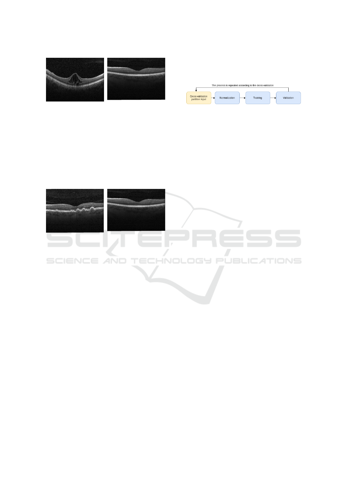
(a) Image of DME (b) Normal image

Figure 2: Example of OCT images divided into normal and

with DME.

1.3 DRUSEN

Optical disc drusen are calciﬁed deposits of extruded

mitochondria that appear in the upper part of the optic

nerve in approximately 2% of the population (Gaier

et al., 2017). In the ﬁgure 3 you can view the OCT

image, divided into normal and DRUSEN.

(a) Image of DRUSEN (b) Normal image

Figure 3: Example of OCT images divided into normal and

with DRUSEN.

2 MATERIALS AND METHODS

In this section, the structure of the adopted systems

will be presented to solve the classiﬁcation of OCT

images, classifying them as, CNV, DME, NORMAL,

DRUSEN, will also be presented the entire structure

of the algorithms as well as the evaluation metrics.

2.1 Structure of the System

The system was divided into three stages, the ﬁrst

consisting of the division and normalization of the

dataset, according to the ﬁgure 4. In the second one

the training was carried out and ﬁnally the data vali-

dation was done. Pre-processing consists of normaliz-

ing the data, the images are in grayscale, all pixels are

divided by 255, to convert them into ﬂoating points.

Represented in the ﬁgure 4 in yellow.

In ﬁgure 4 you can see the process of construc-

tion and training of artiﬁcial neural network model.

In the test data prediction step, the test images that

were separated by the k-fold algorithm are entered,

so accuracy is collected. The process is repeated 5

times, changing the test and training images after the

k-fold calculation.

Figure 4: Construct, training and validate of the models.

2.2 CNN

CNNs are similar to traditional neural networks, both

are composed of neurons that have weights and bias

that need to be trained. Each neuron receives some in-

puts, applies the scalar product of inputs and weights

in addition to a non-linear function (Chen et al.,

2017).

A CNN assumes that all inputs are images, which

allows you to encode some properties in the archi-

tecture. Traditional neural networks are not scalable

for images, since they produce a very high number of

weights to be trained (Esteva et al., 2017).

A CNN consists of a sequence of layers as can

be seen ﬁgure 6, in addition to input layer, which is

usually composed of an image with width and height,

there are three main layers: convolutional layer, pool-

ing layer and fully connected layer. In addition, after

a convolutional layer it is common an activation layer,

normally a linear rectiﬁcation unit function (ReLu)

equations 1, 2. These layers, when sequenced (or

stacked), form an architecture of a CNN (Salamon

and Bello, 2017).

f (x) = x

= max(0,x) (1)

f (x) =

(

0 for x < 0

x for x ≥ 0

(2)

2.2.1 Convolutional Layer

The convolutional layer is the most important layer of

the network, where it carries out the heaviest part of

computational processing. This layer is composed of

a set of ﬁlters (kernels) capable of learning according

to a training (Ustinova et al., 2017). The kernels are

small matrices that in this case was used the size 3x3

to obtain a better precision in the time to go through

the matrix of the images, composed by real values that

can be interpreted as weights.

Given a two-dimensional image, I, and a small ar-

ray, K of size h x w (kernel), the convoked image, I

* K, is calculated by overlapping the kernel at the top

of the image of all possible shapes, and recording the

BIOINFORMATICS 2020 - 11th International Conference on Bioinformatics Models, Methods and Algorithms

170

sum of the elementary products between the image

and the kernel equation 3.

(I ∗ K)

∑

i=1

∑

j=1

i j

x+i−1,y+ j−1

(3)

The kernels are convolved with the input data to

get a feature map. These maps indicate regions in

which speciﬁc features in relation to kernels. The ac-

tual values of the kernels change throughout the train-

ing, causing the network to learn to identify signif-

icant regions to extract characteristics from the data

set (Maggiori et al., 2017), in this way, each ﬁlter

results in an output of a three-dimensional array. In

the convolution results matrices the ReLU activation

function, equations 1, 2 are applied in each element

of the convolution result.

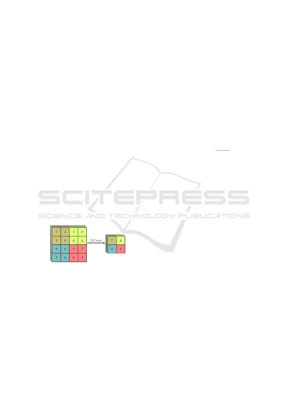
2.2.2 Pooling Layer

After convolution layer exists a pooling layer. The

pooling technique is used to reduce the spatial size of

the resulting convolution matrices, according to the

ﬁgure 5. Consequently, this technique reduces the

amount of parameters to be learned in the network,

contributing to the control of over-ﬁtting, ie avoiding

the condition when a trained model works very well in

training data, but does not work very well in test data

(Yu et al., 2017). The pooling layers operate inde-

pendently on each of the channels of the convolution

result. In addition, you must ﬁrst determine the size

of the ﬁlter to perform pooling.

Figure 5: Example max-pooling with a 4x4 image.

The maximum pool operation reduces the size of

the resource map, this operation can be described by

the equation 4. Let S be the value of the passed and

Q × Q the shape of the feature map before the maxi-

mum grouping and p determines the clustering max-

pooling size (Havaei et al., 2017). The output of the

max-pooling operation would be D × D size.

D = (Q − p)/S + 1 (4)

2.2.3 Fully Connected Layer

The fully connected layer comes after a convolutional

or pooling layer, it is necessary to connect each ele-

ment of the convolution output matrices to an input

neuron. The output of the convolutional and pooling

layers represent the characteristics extracted from the

input image. The purpose of fully-connected layers is

to use these characteristics to classify the image in a

pre-determined class.

The last two layers of the network use the sigmoid

function as the activation function, equation 5. This

function takes a real value and ”transforms” it into

the interval between 0 and 1. In particular, large neg-

ative numbers become 0 and large positive numbers

become 1 (Zaheer and Shaziya, 2018). The sigmoid

function has seen frequent use historically since it has

a good interpretation like the ﬁring rate of a neuron:

from not ﬁring (0) to a fully saturated ﬁring at a pre-

sumed maximum frequency (1) (Zaheer and Shaziya,

2018).

f (x) = sigmoid(x) =

1 + e

−x

(5)

The technique known as dropout is also used in

the fully connected layer to reduce training time and

avoid over-ﬁtting. This technique consists in ran-

domly removing a certain percentage of neurons from

a layer at each training iteration, re-adding them to the

next iteration (Kov

acs et al., 2017).

2.2.4 CNN Architecture

In the ﬁgure 6 the CNN architecture is displayed, it

has 12 layers, where the ﬁrst ten convolutionals layers

and the last two without convolution with the sigmoid

activation function. The input of the network receives

a 150x150 pixel image, each the convolutional layer

has the activation function ReLUs. For the convolu-

tion kernel, the 3x3 size was adopted, because this

way it is possible to have a greater precision in the

time to go through the entire image.

After two convolutional layers a Max-pooling

layer is used, this reduces the size of the matrices re-

sulting from the convolution. With this layer it is pos-

sible to reduce the amount of parameters that will be

learned by the network, this way it is done over ﬁtting

control.

In the latter two the sigmoid activation function

is used, this function is responsible for making the

probabilistic distribution of the input image belong to

each of the classes in which the network was trained.

To reduce the training time and to avoid over-ﬁtting is

used dropout in the layer, ie it is randomly removed at

each training interaction, a certain percentage of the

neurons of a layer, re-adding them in the following

iteration.

Classiﬁcation of Optical Coherence Tomography using Convolutional Neural Networks

171

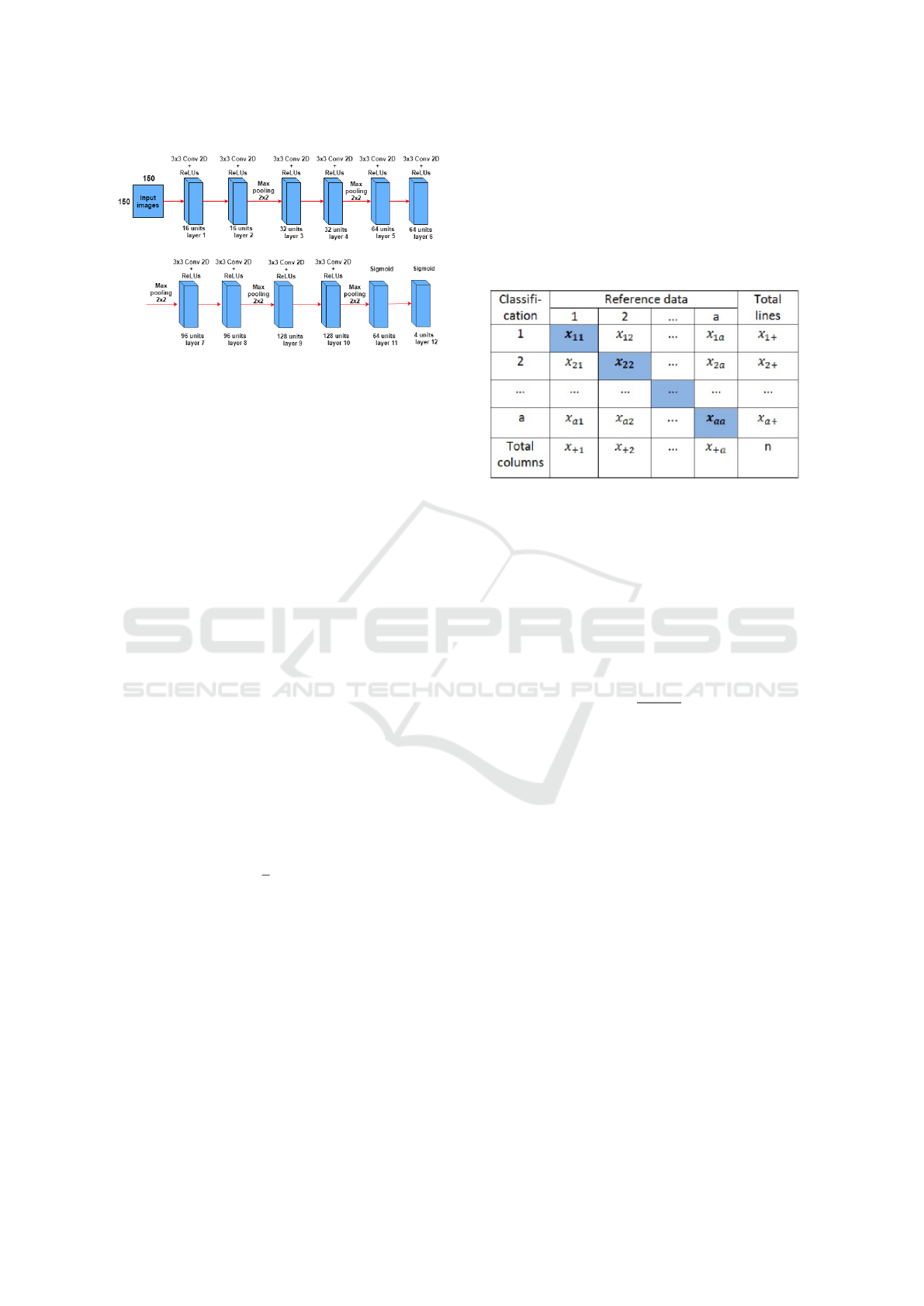
Figure 6: Construction of the CNN training mode.

3 METRICS OF THE

EVALUATION

3.1 Cross Validation

Cross-validation is an evaluation technique on the

ability of generalization models, from a dataset, is

widely used in problems where the object is the mod-

eling and prediction (Vehtari et al., 2017). With this it

is possible to estimate how precise the model is, that

is, its accuracy with data that it does not know.

The k-fold cross-validation method consists of di-

viding the total set into k subsets of the same size.

One subset is used for testing, and the other k-1 sub-

sets for training. This process is repeated by k times,

if circularly changing the subset of tests (Grimm et al.,

2017).

The ﬁnal precision of the model is estimated by

equation 6, at where Ac

is the sum of the differences

between the actual value y

and the predicted value

ˆy

e k is the amount of k-fold divisions. With this it

is possible to infer the generalization capacity of the

network.

∑

i=1

− ˆy

) (6)

3.2 Confusion Matrix

As a statistical tool we have the confusion matrix that

provides the basis for describe the accuracy of the

classiﬁcation and characterize the errors, helping re-

ﬁne the ranking (Saraiva et al., 2018).The confusion

matrix is formed by an array of squares of numbers

arranged in rows and columns that express the num-

ber of sample units of a particular category, inferred

by a decision rule, compared to the category current

ﬁeld.

Usually below the columns is the set reference

data that is compared to the product data of the classi-

ﬁcation that are represented along the lines. The ﬁg-

ure 7 shows the representation of an array of confu-

sion. The elements of the main diagonal in bold indi-

cate the level of accuracy, or agreement, between the

two sets of data.

Figure 7: Example matrix of confusion.

The measures derived from the confusion ma-

trix are: the total accuracy being that chosen by the

present work, accuracy of individual class, producer

precision, user precision and Kappa index, among

others. The total accuracy is calculated by dividing

the sum of the main diagonal of the error matrix x

by the total number of samples collected n. Accord-

ing to the equation 7.

T =

∑

(7)

4 RESULTS

In this section will be presented the classiﬁcation per-

formance results of the training model. The metrics

used to evaluate the results are: The average accu-

racy of the cross validation, speciﬁcity and sensitivity,

given by the ROC curve.

In the table 1 the results obtained by the training

network are presented. through the table it is possible

to extract information such as: False positives, False

negatives, True positives, True Negative and accuracy

of each interaction of cross validation. The average

accuracy of the network was 94.35%.

In the ﬁgure 9 it is possible to check the data re-

lating to iteration 5 of the table 1. In it is shown a

conﬂuence matrix, a graph of the ROC curve and the

precision recall curve. Where it is possible to visual-

ize the sensitivity and speciﬁcity of each class. It is

possible to visualize in the ﬁgure 8 the graphs of pro-

portions, of each disease and of the test and training.

BIOINFORMATICS 2020 - 11th International Conference on Bioinformatics Models, Methods and Algorithms

172

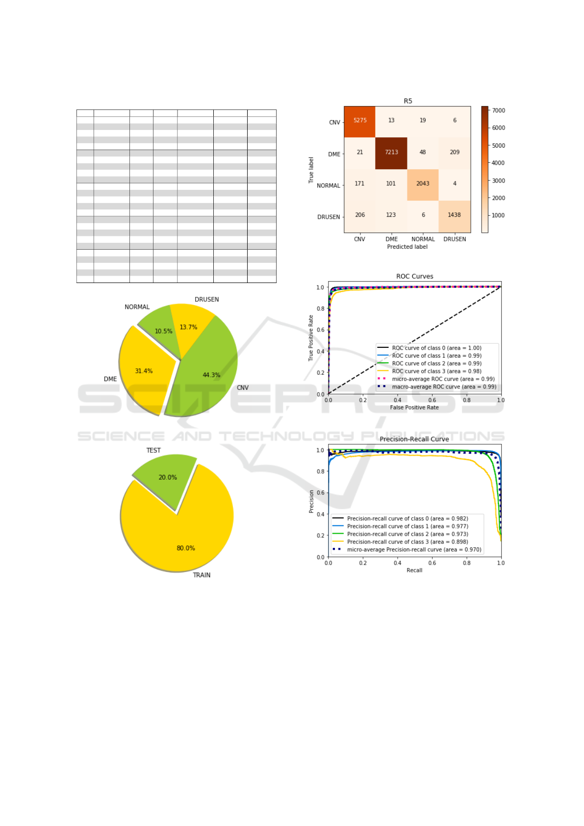
Table 1: Table of iterations and classiﬁcations.

** CNV DME NORMAL DRUSEN ACC

1 CNV 5274 10 19 10

1 DME 38 7247 77 83

1 NORMAL 2017 63 2045 5

1 DRUSEN 193 229 9 1343

1 ACC 94.44%

2 CNV 5087 14 168 44

2 DME 9 7329 47 106

2 NORMAL 7 96 2148 6

2 DRUSEN 126 212 22 1413

2 ACC 94.55%

3 CNV 5252 12 22 27

3 DME 17 7348 19 107

3 NORMAL 176 118 2014 12

3 DRUSEN 138 172 2 1461

3 ACC 95.13%

4 CNV 5253 9 8 43

4 DME 58 7130 56 247

4 NORMAL 390 71 1831 27

4 DRUSEN 160 79 7 1527

4 ACC 93.16%

5 CNV 5275 13 19 06

5 DME 21 7213 48 209

5 NORMAL 171 101 2043 4

5 DRUSEN 206 123 6 1438

5 ACC 94.51%

(a) Proportion of the dataset between training and validation

(b) Demographics Proportion Chart

Figure 8: Demographics Proportion Chart.

It is worth noting that the test and training data were

separated proportionally to their total quantity.

Neural network training was performed using an

NVIDIA GTX 1060 video card, which features 1280

CUDA cores (processors), 6 GB of dedicated mem-

ory, 12 GB of RAM and a fourth-generation Core i5

Processor with time of training of 29 minutes.

(a) Confusion matrix

(b) ROC curves

Figure 9: Interaction test 5 table 1, Precision recall curve

and ROC curves.

5 CONCLUSION

In this work, a model was presented to classify visi-

ble pathologies in OCT, the classes are CNV, DME,

DRUSEN and NORMAL. For the validation of the

models, cross validation was performed, where it is

Classiﬁcation of Optical Coherence Tomography using Convolutional Neural Networks

173

possible to verify the generalization capacity. The

classiﬁcation model evaluated in this work was shown

to be efﬁcient, obtaining an average of 94.35 % ac-

curacy. Being able to reach a high accuracy, even

with the unbalanced dataset and with the iterations

obtained in the cross validation being proxies.

ACKNOWLEDGMENTS

The elaboration of this work would not have been

possible without the collaboration of the Engineering

and DecisionSupport Research Center (GECAD) of

the Institute of Engineering, Polytechnic Institute of

Porto, Portugal and FAPEMA.

REFERENCES

Alten, F., Lauermann, J., Clemens, C., Heiduschka, P.,

and Eter, N. (2017). Signal reduction in chorio-

capillaris and segmentation errors in spectral domain

oct angiography caused by soft drusen. Graefe’s

Archive for Clinical and Experimental Ophthalmol-

ogy, 255(12):2347–2355.

Baxter, S. L., Pistilli, M., Pujari, S. S., Liesegang, T. L.,

Suhler, E. B., Thorne, J. E., Foster, C. S., Jabs,

D. A., Levy-Clarke, G. A., Nussenblatt, R. B., et al.

(2013). Risk of choroidal neovascularization among

the uveitides. American journal of ophthalmology,

156(3):468–477.

Bressler, S. B., Glassman, A. R., Almukhtar, T., Bressler,

N. M., Ferris, F. L., Googe Jr, J. M., Gupta, S. K., Jam-

pol, L. M., Melia, M., Wells III, J. A., et al. (2016).

Five-year outcomes of ranibizumab with prompt or

deferred laser versus laser or triamcinolone plus de-

ferred ranibizumab for diabetic macular edema. Amer-

ican journal of ophthalmology, 164:57–68.

Chen, Y.-H., Krishna, T., Emer, J. S., and Sze, V. (2017).

Eyeriss: An energy-efﬁcient reconﬁgurable acceler-

ator for deep convolutional neural networks. IEEE

Journal of Solid-State Circuits, 52(1):127–138.

Dimitrova, G., Chihara, E., Takahashi, H., Amano, H., and

Okazaki, K. (2017). Quantitative retinal optical co-

herence tomography angiography in patients with dia-

betes without diabetic retinopathy. Investigative oph-

thalmology & visual science, 58(1):190–196.

Esteva, A., Kuprel, B., Novoa, R. A., Ko, J., Swetter, S. M.,

Blau, H. M., and Thrun, S. (2017). Dermatologist-

level classiﬁcation of skin cancer with deep neural net-

works. Nature, 542(7639):115.

Gaier, E. D., Rizzo III, J. F., Miller, J. B., and Ces-

tari, D. M. (2017). Focal capillary dropout asso-

ciated with optic disc drusen using optical coher-

ence tomographic angiography. Journal of Neuro-

ophthalmology, 37(4):405–410.

Gill, A., Cole, E. D., Novais, E. A., Louzada, R. N., Carlo,

T., Duker, J. S., Waheed, N. K., Baumal, C. R., and

Witkin, A. J. (2017). Visualization of changes in the

foveal avascular zone in both observed and treated di-

abetic macular edema using optical coherence tomog-

raphy angiography. International journal of retina and

vitreous, 3(1):19.

Grimm, K. J., Mazza, G. L., and Davoudzadeh, P. (2017).

Model selection in ﬁnite mixture models: A k-fold

cross-validation approach. Structural Equation Mod-

eling: A Multidisciplinary Journal, 24(2):246–256.

Havaei, M., Davy, A., Warde-Farley, D., Biard, A.,

Courville, A., Bengio, Y., Pal, C., Jodoin, P.-M., and

Larochelle, H. (2017). Brain tumor segmentation

with deep neural networks. Medical image analysis,

35:18–31.

Kermany, D., Zhang, K., and Goldbaum, M. (2018). La-

beled optical coherence tomography (oct) and chest

x-ray images for classiﬁcation. Structural Equation

Modeling: A Multidisciplinary Journal.

Kov

acs, G., T

oth, L., Van Compernolle, D., and Ganapathy,

S. (2017). Increasing the robustness of cnn acoustic

models using autoregressive moving average spectro-

gram features and channel dropout. Pattern Recogni-

tion Letters, 100:44–50.

Maggiori, E., Tarabalka, Y., Charpiat, G., and Alliez, P.

(2017). Convolutional neural networks for large-scale

remote-sensing image classiﬁcation. IEEE Transac-

tions on Geoscience and Remote Sensing, 55(2):645–

657.

Parhi, K. K., Reinsbach, M., Koozekanani, D. D., and Roy-

chowdhury, S. (2017). Automated oct segmentation

for images with dme. In Medical Image Analysis and

Informatics, pages 115–132. CRC Press.

Preti, R. C., Govetto, A., Aqueta Filho, R. G., Zacharias,

L. C., Pimentel, S. G., Takahashi, W. Y., Monteiro,

M. L., Hubschman, J. P., Sarraf, D., et al. (2018). Op-

tical coherence tomography analysis of outer retinal

tubulations: sequential evolution and pathophysiolog-

ical insights. Retina, 38(8):1518–1525.

Roy, R., Saurabh, K., Bansal, A., Kumar, A., Majum-

dar, A. K., and Paul, S. S. (2017). Inﬂammatory

choroidal neovascularization in indian eyes: Etiology,

clinical features, and outcomes to anti-vascular en-

dothelial growth factor. Indian journal of ophthalmol-

ogy, 65(4):295.

Salamon, J. and Bello, J. P. (2017). Deep convolutional neu-

ral networks and data augmentation for environmental

sound classiﬁcation. IEEE Signal Processing Letters ,

24(3):279–283.

Saraiva, A., Melo, R., Filipe, V., Sousa, J., Ferreira, N. F.,

and Valente, A. (2018). Mobile multirobot manipula-

tion by image recognition.

Saraiva., A. A., Ferreira., N. M. F., de Sousa., L. L., Costa.,

N. J. C., Sousa., J. V. M., Santos., D. B. S., Valente.,

A., and Soares., S. (2019a). Classiﬁcation of images

of childhood pneumonia using convolutional neural

networks. In Proceedings of the 12th International

Joint Conference on Biomedical Engineering Systems

and Technologies - Volume 2: BIOIMAGING,, pages

112–119. INSTICC, SciTePress.

Saraiva., A. A., Santos., D. B. S., Costa., N. J. C., Sousa.,

J. V. M., Ferreira., N. M. F., Valente., A., and Soares.,

BIOINFORMATICS 2020 - 11th International Conference on Bioinformatics Models, Methods and Algorithms

174

S. (2019b). Models of learning to classify x-ray im-

ages for the detection of pneumonia using neural net-

works. In Proceedings of the 12th International Joint

Conference on Biomedical Engineering Systems and

Technologies - Volume 2: BIOIMAGING,, pages 76–

83. INSTICC, SciTePress.

Schlanitz, F. G., Baumann, B., Kundi, M., Sacu, S., Barat-

sits, M., Scheschy, U., Shahlaee, A., Mitterm

uller,

T. J., Montuoro, A., Roberts, P., et al. (2017). Drusen

volume development over time and its relevance to the

course of age-related macular degeneration. British

Journal of Ophthalmology, 101(2):198–203.

Sivaprasad, S. and Moore, A. (2008). Choroidal neovascu-

larisation in children. British Journal of Ophthalmol-

ogy, 92(4):451–454.

Swanson, E. A. and Fujimoto, J. G. (2017). The ecosystem

that powered the translation of oct from fundamental

research to clinical and commercial impact. Biomedi-

cal optics express, 8(3):1638–1664.

Ustinova, E., Ganin, Y., and Lempitsky, V. (2017). Multi-

region bilinear convolutional neural networks for per-

son re-identiﬁcation. In Advanced Video and Signal

Based Surveillance (AVSS), 2017 14th IEEE Interna-

tional Conference on, pages 1–6. IEEE.

Vehtari, A., Gelman, A., and Gabry, J. (2017). Prac-

tical bayesian model evaluation using leave-one-out

cross-validation and waic. Statistics and Computing,

27(5):1413–1432.

Wells, J. A., Glassman, A. R., Ayala, A. R., Jampol, L. M.,

Bressler, N. M., Bressler, S. B., Brucker, A. J., Fer-

ris, F. L., Hampton, G. R., Jhaveri, C., et al. (2016).

Aﬂibercept, bevacizumab, or ranibizumab for diabetic

macular edema: two-year results from a comparative

effectiveness randomized clinical trial. Ophthalmol-

ogy, 123(6):1351–1359.

Yu, S., Jia, S., and Xu, C. (2017). Convolutional neural

networks for hyperspectral image classiﬁcation. Neu-

rocomputing, 219:88–98.

Zaheer, R. and Shaziya, H. (2018). Gpu-based empiri-

cal evaluation of activation functions in convolutional

neural networks. In 2018 2nd International Confer-

ence on Inventive Systems and Control (ICISC). IEEE.

Classiﬁcation of Optical Coherence Tomography using Convolutional Neural Networks

175