Neural Network Security: Hiding CNN Parameters with Guided

Grad-CAM

Linda Guiga

1,∗

and A. W. Roscoe

IDEMIA and T

ecom ParisTech, Paris, France

Department of Computer Science, University of Oxford, Oxford, U.K.

Keywords:

CNN, Security, Reverse-engineering, Grad-CAM, Parameter Protection.

Abstract:

Nowadays, machine learning is prominent in most research ﬁelds. Neural Networks (NNs) are considered

to be the most efﬁcient and popular architecture nowadays. Among NNs, Convolutional Neural Networks

(CNNs) are the most popular algorithms for image processing and image recognition. They are therefore

widely used in the industry, for instance for facial recognition software. However, they are targeted by several

reverse-engineering attacks on embedded systems. These attacks can potentially ﬁnd the architecture and

parameters of the trained neural networks, which might be considered Intellectual Property (IP). This paper

introduces a method to protect a CNN’s parameters against one of these attacks (Tram

er et al., 2016). For

this, the victim model’s ﬁrst step consists in adding noise to the input image so as to prevent the attacker from

correctly reverse-engineering the weights

1 INTRODUCTION

Deep learning is ever more important, touching most

research areas. Among deep learning models, Con-

volutional Neural Networks (CNNs) are often used

when it comes to image processing and classiﬁcation

(Krizhevsky et al., 2012; Coskun et al., 2017). For

this reason, CNNs can be found on many embedded

systems from our daily lives - such as smartphones.

Face ID, the face recognition feature on the IPhone

X, is an example (Inc., 2017).

Because of the efﬁciency of CNNs in image clas-

siﬁcation and processing, industry makes much use

of them. This entails two security problems: it is nec-

essary to protect the companies’ intellectual property

(IP) and to ensure the output has not been tampered

with. Indeed, since ﬁnding the optimal architecture

and parameters for a CNN require much time and

computational power, the model used is part of the

company’s IP and should be kept safe from potential

malicious competitors. Second, for some applications

- such as face recognition - it must be infeasible to ﬁnd

an input on which the output is incorrect. Learning

the parameters of the embedded CNN can turn such a

problem from infeasible to feasible.

In the case of face recognition, for instance, an

∗

Work conducted at the University of Oxford.

attacker who can manipulate the output of a model

could impersonate someone and steal, for instance,

the data on a mobile phone (Sharif et al., 2016; Deb

et al., 2019; Dong et al., 2019).

Unfortunately, CNNs are the target to many differ-

ent attacks. The most common attacks are adversarial

ones. The goal of an adversarial attack is to change

the model’s output for some selected inputs, without

changing the predictions for the other inputs. This is

the basis of the impersonation attacks in (Dong et al.,

2019). Since adversarial attacks are made easier if

the attacker knows the model’s parameters and archi-

tecture (Akhtar and Mian, 2018), protecting them is

paramount.

However, multiple reverse-engineering attacks

can potentially extract the victim model’s key param-

eters (Tram

er et al., 2016; Oh et al., 2018).

In that context, this paper aims at protecting CNNs

against equation-solving reverse-engineering attacks

(Tram

er et al., 2016) by adding noise to the input, us-

ing visualization maps. Its main contribution is the

use of random noise as a way of protecting the pa-

rameters against reverse-engineering attacks - rather

than protecting the input data or increasing accuracy.

The ﬁrst section of this paper describes the neces-

sary background for the method. In the second sec-

tion, we detail our proposed method. In the last sec-

tion, we explain our experiments and show the efﬁ-

Guiga, L. and Roscoe, A.

Neural Network Security: Hiding CNN Parameters with Guided Grad-CAM.

DOI: 10.5220/0009061206110618

In Proceedings of the 6th International Conference on Information Systems Security and Privacy (ICISSP 2020), pages 611-618

ISBN: 978-989-758-399-5; ISSN: 2184-4356

611

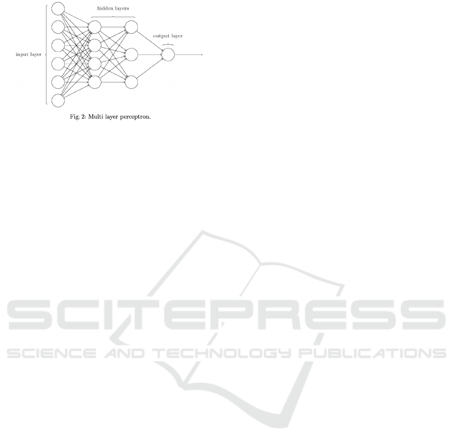
Figure 1: Multi Layer Perceptron (Image taken from

(Batina et al., 2019)).

ciency of our method against Tram

er et al.’s equation-

solving attack.

2 BACKGROUND AND RELATED

WORK

In this section, we describe neural networks, detail

an attack on the parameters of a neural network and

explain Guided Grad-CAM, a visualization mapping

we will use in our defence.

2.1 Neural Networks

A neural network (NN) model can be described as a

function f : X →Y ∈ [0, 1]

where c is the number of

classes in the model. It is often composed of several

layers of different types. A Multi Layer Perceptron

(MLP) is a NN only composed of fully-connected lay-

ers: each neuron in one layer is connected to all neu-

rons in the next layer, with a certain weight w (see

Fig. 1). Multiclass Logistic Regressions (MLRs) are

NNs that classify data into c different classes.

CNNs - often used in image classiﬁcation - are

NNs with mainly convolutional layers. These lay-

ers compute a convolution between ﬁlters F- 2-

dimensional matrices smaller than the input of the

layer - and the input of the layer. The elements of

the ﬁlters are the weights of the layer. In most cases,

a pooling layer, which performs a down-sampling

of their input, follows convolutional layers (Scherer

et al., 2010).

The weights are learnt through the optimization of

a loss function. The most common one for CNNs is

the categorical cross entropy (Srivastava et al., 2019).

This optimization of a loss function is done over sev-

eral runs - or epochs -, on a chosen dataset - the train-

ing set. This optimization problem is often solved

using either Stochastic Gradient Descent (SGD) with

Nesterov Momentum (Bengio et al., 2012) or Adam

(Kingma and Ba, 2017), as they usually perform bet-

ter than other optimizers.

2.2 Attack on Parameters

In 2016, Tram

er et al. (Tram

er et al., 2016) de-

scribed several attacks on Machine Learning models.

For neural networks, the authors described equation-

solving and retraining attacks on small models. The

retraining approaches required a much higher query-

ing budget (×20) than the equation-solving attacks.

In the context of CNNs, which have tens of thou-

sands of parameters for small architectures, retraining

attacks induce tremendous overhead. Thus, in what

follows, we will only consider the equation-solving

attack given the conﬁdence values.

In Tram

er et al.’s equation-solving attack, the at-

tacker knows the victim model’s architecture, and can

make as many queries to the model as necessary: their

attacker randomly generates a set of query inputs, and

receives the corresponding outputs. This provides

them with a non-linear system of equations of the

form:

f (x

) = y

∀i ∈ {1, ..., b}

(1)

where b is the size of the generated input set.

The attacker then creates a new model with the

same architecture as the victim model’s and optimizes

a categorical cross entropy loss function with the vic-

tim model’s probability distribution - corresponding

to the y

queried beforehand - as the target distribu-

tion. This attack was successfully applied on MLRs

and MLPs by Tram

er et al. In this paper, we try to

protect CNNs against this attack on the last layer of

the model.

2.3 Guided Grad-CAM

Not all neurons in a CNN have the same impact on

predictions. Some works (Mahendran and Vedaldi,

2016) have asserted that the last layers of an image

focus more on the global characteristics and tend to

discard more details than the ﬁrst ones. Thus, the

analysis of the neurons used in those last convolu-

tional layers might help determine the most relevant

parts of an image for the NN’s prediction.

The goal of visualization techniques such as

saliency (K. Simonyan and Zisserman, 2014), Guided

Backpropagation (J. T. Springenberg and Riedmiller,

2014) or Class Activation Maps (CAM) (Zhou et al.,

2015) is to show the way the model makes its predic-

tions. Indeed, given an image and a class label, they

return a visualization of the parts of the image associ-

ated - according to the model - to the class label (see

Fig. 3a and 3b in Sec. 4).

ICISSP 2020 - 6th International Conference on Information Systems Security and Privacy

612

Guided Grad-CAM (Selvaraju et al., 2016) uses

the gradients received at the last convolutional layer in

order to compute such a visualization map. These gra-

dients are closely related to the importance weights

of the corresponding pixels. The importance weight

of a pixel evaluates the impact a change in the pixel

would have on the prediction. Guided Grad-CAM

corresponds to a mix of Guided Backpropagation and

a generalized version of CAM, Grad-CAM, and is re-

sistant to adversarial attacks (Selvaraju et al., 2016):

even though imperceptible noise is added to the im-

age - leading to a wrong prediction -, the localization

maps remain unchanged.

2.4 Related Works

Adding noise to the input of a model during the train-

ing phase is common practice. Indeed, it helps im-

prove the accuracy and the generalizability of the

model trained (An, 1996; Bishop, 1995). If no noise

or regularization term is added, the training leads to

an overﬁtting over the training data. Some papers also

consider adding noise to the output of some layers

or to the gradients during backpropagation to achieve

a better accuracy and/or a faster convergence (Nee-

lakantan et al., 2015; Audhkhasi et al., 2016). How-

ever, our defence does not consider the training phase:

we only add noise during inference.

It is also interesting to note that noise injection

can be used to defend against adversarial examples,

and therefore to improve the NN’s robustness. Gu and

Rigazio add Gaussian noise and then use an autoen-

coder to remove it as a way of detecting adversarial

examples (Gu and Rigazio, 2014).

Additive noise is also a common protection tool.

Indeed, making a mechanism differentially private

usually consists in adding noise to the output of the

function to protect. This is, for instance, applied to

the Stochastic Gradient Descent (SGD) during the

training phase of a model to avoid leaking training

data (Abadi et al., 2016). Since differential privacy

provides security guarantees, Shokri and Shmatikov

apply it to joint learning of NN models: their pa-

per enables participants to jointly train a model by

sharing the parameter updates with the other partic-

ipants without leaking any information about their se-

cret dataset (Shokri and Shmatikov, 2015).

However, our goal is different from the works

mentioned above. Adding noise to the input has not

been used to protect the parameters of a model. More-

over, visualization maps have not previously been ap-

plied to the selection of ‘unimportant’ pixels as sug-

gested in this paper. In that sense, the method pro-

posed here is believed to be original and introduces

another use of saliency and visualization maps.

3 PROTECTING THE WEIGHTS:

METHOD DESCRIPTION

This section details the threat model considered, as

well as the method used to protect against the attack

described in Sec. 2.2.

3.1 Threat Model

If no prior knowledge about the victim model - such

as the architecture - is supposed, then an attacker try-

ing to extract weights from a model needs to train sev-

eral models from a - usually reduced - search space

(Oh et al., 2018). Let us note that if the architec-

ture is not known, it may be correctly guessed (Hong

et al., 2018; Yan et al., 2018). Another option for

such an attacker would be to conduct side-channel at-

tacks, such as in (Batina et al., 2019). In our case, we

will assume a stronger attacker, who already knows

the architecture of the model. This is a plausible sce-

nario given the various attacks on the architectures of

CNNs (Batina et al., 2019; Yan et al., 2018; Hong

et al., 2018).

Therefore, our threat model is the same as the one

in Tram

er et al.’s paper (Tram

er et al., 2016):

• The attacker knows the architecture of the victim

model.

• The attacker can query the victim model as many

times as necessary. This means that the attacker

can have at their disposal a set of pairs (x, f (x))

where x is in the input space, and f (x) is its cor-

responding conﬁdence values.

The goal of the attacker is to extract the parameters -

here, essentially the weights - of a CNN. The original

attack by Tram

er et al. extracted all of the model’s

parameters. However, we limited our study to the last

layer of CNNs, due to their high number of parame-

ters.

3.2 Adding Noise to the Input

The method proposed to protect the weights is to add

random noise to the input image during the inference

phase. Adding small amounts of noise can highlight

the important features and improve the model’s accu-

racy. On the other hand, adding too much noise leads

to a drop in the victim model’s accuracy. Thus, the

challenge here is to add enough noise without alter-

ing the model’s predictions.

Neural Network Security: Hiding CNN Parameters with Guided Grad-CAM

613

With noisy inputs, the attacker gets a set of pairs

(x, f (x

)) where x

:= x+ n for some noise n unknown

to the attacker, resulting in noisy extracted weights w

for the attacker.

The noise we will consider is a normal distribu-

tion over a selected set S of pixels, with either a high

expected value - leading to a noisy output by linearity

- or a high standard deviation. Batch normalization

(BN) - a normalize layer - was introduced in 2015 by

S. Ioffe and C. Szegedy to limit the change of distri-

bution in the input during training, and therefore im-

prove its speed, performance and stability (Ioffe and

Szegedy, 2015). For each element x

i, j

in the input, the

layer computes:

i, j

−µ

batch

√

batch

+ε

(2)

where µ

batch

is the expected value of a given batch,

batch

is its variance and ε is a small positive value

added in order to avoid division by 0.

Eq. 2 shows that the output of the BN layer is in-

versely proportional to the batch’s standard deviation.

Thus, adding noise with a high standard deviation de-

creases the dependence of the output with the original

input values.

In order to add enough noise to alter the attacker’s

extracted weights without altering the victim model’s

predictions, we selected a set S of pixels considered

to be “unimportant” to the model’s predictions, and

only added noise to those pixels. To do so, we com-

puted the visualization map thanks to Guided Grad-

CAM (Selvaraju et al., 2016) and set a threshold t. All

neurons whose importance weights - in other words,

whose value after Guided Grad-CAM was applied -

are below t are selected to receive noise.

4 EXPERIMENTS

In this section, we detail the experiments carried on in

order to select the set S of pixels we added noise to.

We also explain the way the attack and defence were

set up, and the results of the various experiments.

4.1 Selection of Pixels

Let us start this section by explaining the way we se-

lected the pixels to modify in the input image using

Grad-CAM.

The code used to run Guided Grad-CAM consists

in a slight modiﬁcation of the code found in (Gilden-

blat, 2017).

For clarity, let us consider the VGG19 architecture

(Simonyan and Zisserman, 2014), for which Guided

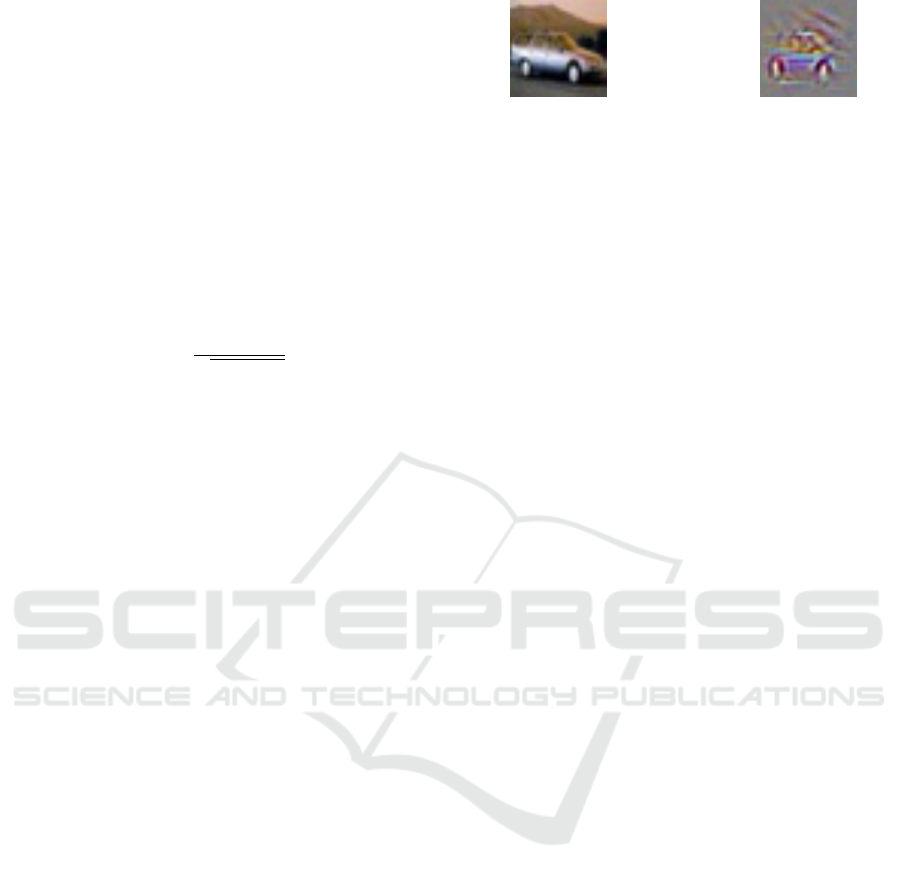
(a) Image of a car from

the CIFAR10 dataset

(b) Guided Grad-CAM

Figure 2: Visualization map resulting from Guided Grad-

CAM applied to the image of a car from the CIFAR10

dataset, with the LeNet architecture.

Grad-CAM performs well. Let grad denote the output

image of the Guided Grad-CAM algorithm. Let t de-

note the threshold we choose to select the “unimpor-

tant indices”. Let m be the maximum value in grad.

Finally, let p denote the value of a pixel after Guided

Grad-CAM was performed. Then, the selected pixels

are such that 0 ≤ p < t ×m. For the VGG19 archi-

tecture, the noise we added to the selected pixels is a

normal distribution with expected value µ = 125 and

standard deviation σ = 25.

The following paragraphs explain the way we set

the threshold t.

Choosing t = 0.25 results in the images in Fig. 3.

With the chosen threshold and noise, the model’s pre-

dictions remain “African Elephant”, with 1,038 pixels

modiﬁed.

Since the predictions are unchanged, we can

choose a higher threshold: t = 0.42 for instance, re-

sulting in 5, 820 chosen pixels. The predictions re-

main intact, but the model is less certain about its pre-

dictions: the probability of the corresponding class

(“African elephant”), lowers from 99.5% to, on aver-

age, 55.97%.

However, selecting the pixels close to half the

maximal value - where the background pixels should

be - results in mostly wrong predictions (around 97%

of wrong predictions).

We give an example of a run of Guided Grad-

CAM on ﬁve images in Fig. 4, with various thresh-

olds. Table 1 summarizes the results depending on

the threshold t chosen. Even though the impact of

the noise varies greatly depending on the image, a

threshold of t = 0.25 enables all predictions to remain

correct, hence a choice of t = 0.25 to minimize the

changes in the model’s predictions.

Let us now consider the case of LeNet, the ﬁrst

CNN, introduced in 1998 by Lecun et al.(Y. LeCun

and Haffner, 1998). Due to the limited depth of the

architecture, guided Grad-CAM does not perform as

well as on larger architectures such as VGG16 or

VGG19 (Simonyan and Zisserman, 2014). However,

it still outlines the important features of a class in the

input image, as is shown in Fig. 2. In what fol-

lows, the “accuracy rate” will be deﬁned as the per-

ICISSP 2020 - 6th International Conference on Information Systems Security and Privacy

614

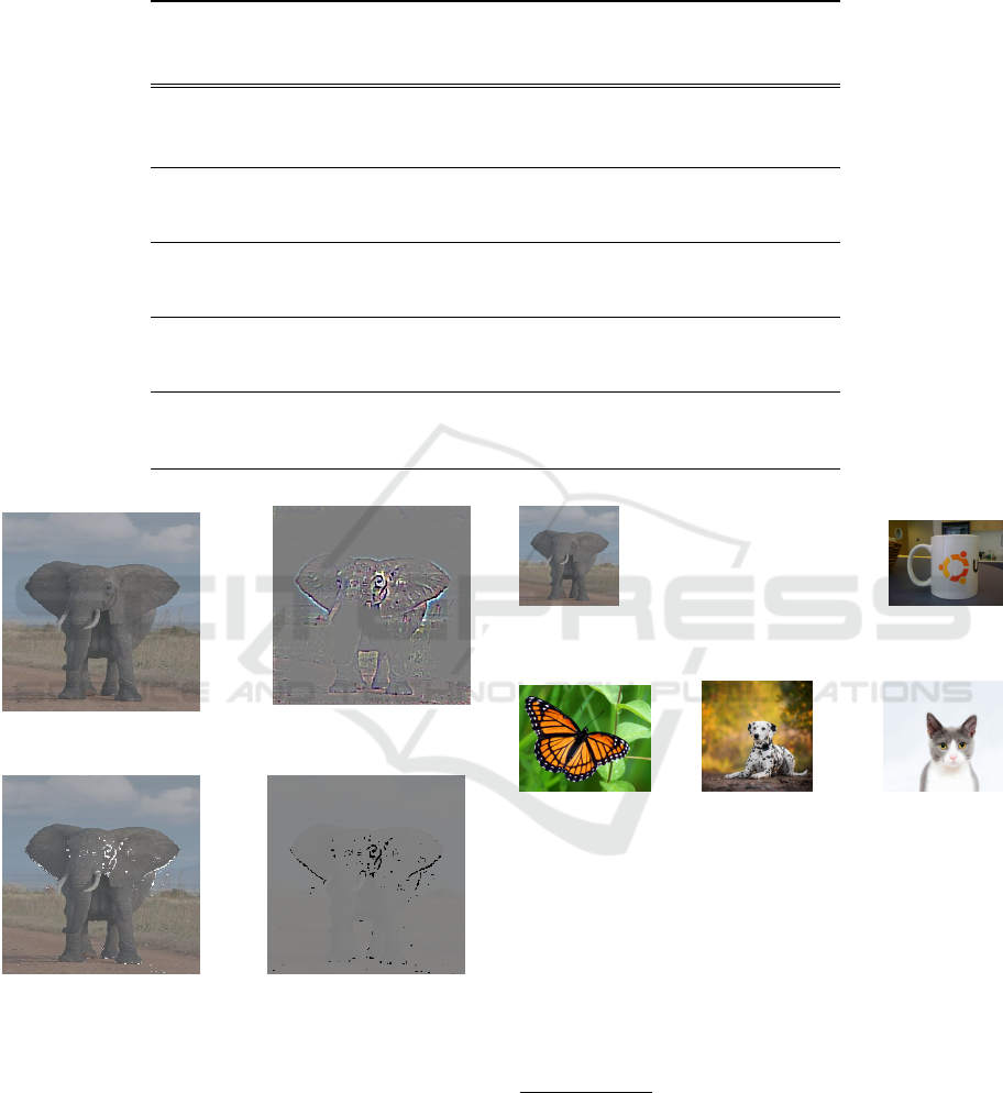
Table 1: Inﬂuence of the noise added with µ = 125 and σ = 25 depending on the threshold t. The selected pixels have a

value p in Guided Grad-CAM such that 0 ≤ p < t ×max(grad). The average class probability corresponds to the average

probability associated to the correct class label over 100 trials.

Image Threshold t

Number

of pixels

changed

Predictions

unchanged

Initial

class

probabil-

ity

Average class

probability

African elephant

0.25 1,038 100%

99.48 %

98.92 %

0.3 1,515 100% 95.53 %

0.4 4,109 100% 95.28 %

0.42 5,820 100% 57.01%

Coffee Mug

0.25 1,815 100%

89.09 %

59.79%

0.3 2,491 85% 39.28 %

0.4 5,593 0% 0 %

0.42 7,546 0% 0 %

Monarch butterﬂy

0.25 1,905 100%

99.75 %

95.44 %

0.3 4,726 100% 86.05 %

0.4 7,894 100% 71.27 %

0.42 10,440 86% 36.63 %

Dalmatian

0.25 1,198 100%

99.8 %

80.22 %

0.3 1,496 100% 63.74 %

0.4 2,623 0% 4.97 %

0.42 2,222 0% 0 %

Egyptian cat

0.25 1,326 100%

42.29 %

58.66 %

0.3 1,657 100% 43.35 %

0.4 2,946 0% 0 %

0.42 3,533 0% 0 %

(a) Original image

(b) Guided Grad-CAM

(grad)

Figure 3: Result of adding a noise with µ = 125 and σ = 25

to the pixels whose value p in the Guided Grad-CAM map

is such that 0 ≤ p < t ×max(grad) where t = 0.25.

centage of predictions that are equal to the victim

model’s original predictions. The noise added to the

chosen pixels has an expected value of 0.8 (represent-

ing around 37.6% of the maximal value), and a stan-

dard deviation of 0.1 (representing around 4.7% of the

maximum value). Similarly to the case of VGG19, we

observed that a threshold of t = 0.25 resulted in un-

changed predictions most of the time.

(a) African

elephant

(b) Coffee

mug

butterﬂy

(d) Dalma-

tian

(e) Egyptian

cat

Figure 4: Images used for VGG19 predictions.

On the ﬁrst 2, 000 images of the CIFAR10 training

set, this threshold leads, on average, to a modiﬁca-

tion of 2% of the pixels and an accuracy of 82%.

This accuracy rate is above the one we get when we

add noise to the whole image (around 79.8%). The

drop in the accuracy rate can however be explained

by LeNet’s low prediction accuracy on CIFAR10 (the

https://en.wikipedia.org/wiki/Elephant#/media/File:

African Bush Elephant.jpg.

https://github.com/Sanghyun-Hong/DeepRecon/

tree/master/etc.

https://www.4ritter.com/events-1/hummingbird

butterﬂy-gardening.

http://goodupic.pw/dog.html.

https://www.pexels.com/photo/adorable-animal

animal-photography-blur-259803/.

Neural Network Security: Hiding CNN Parameters with Guided Grad-CAM

615

Figure 5: Last 8,500 epochs of SGD with Nesterov Mo-

mentum and Adam optimizersThe attack on weights is run

on the the original LeNet architecture. We chose a budget

query of 5,100 and ran the attack for 10,000 epochs.

model we trained had a 62% accuracy) and Guided

Grad-CAM’s reduced efﬁciency on LeNet. In Sec.

3.2, we also explained the inﬂuence of the noise on

an architecture with a BN layer. Thus, we also stud-

ied a LeNet architecture where we added a BN layer

after the ﬁrst convolution. For this architecture, we

kept the threshold of t = 0.25 and we switched the

values of σ and µ: µ = 0.1 and σ = 0.8. The accuracy

of the model increased, as 89.5 % of the predictions

were the same as the original model, yet only around

1.8 % of the pixels changed.

4.2 Attack on Weights

We applied Tram

er et al.’s attack on the last layer of a

LeNet architecture, as well as a simpliﬁed LeNet ar-

chitecture with only 6 ﬁlters instead of 16 in the ﬁrst

convolutional layer. The high accuracy rate Tram

et al. reached on MLRs and MLPs only required

1,000 epochs (they extracted 2,225 parameters with

a 99.8% accuracy for a query budget of 4, 450). Due

to the large number of parameters in LeNet (62,006

for the original LeNet architecture), we focused our

attack on the last dense layer. We show that the ex-

traction of the weights can already be prevented if the

attacker knows all the parameters except those in that

last layer.

We chose Adam as an optimizer, since it pro-

vided a better accuracy on the extracted weights in

the longer run, as can be seen in Fig. 5 .

Let us deﬁne the metric for the evaluation of the

attack.

E( f ,

f ) =

∑

x∈D

d( f (x),

f (x))

|D|

var

( f ,

f ) =

∑

x∈D

var

( f (x),

f (x))

|D|

(3)

where f is the victim model,

f is the extracted model

and D is a test set.

The distance d is deﬁned as follows: d(x, y) = 0

if argmax( f (x)) = argmax( f (y)) and d(x, y) = 1 oth-

erwise. On the other hand, d

var

is the total variation

distance: d

var

(x, y) =

∑

i=0

−y

| where c is the

number of classes. For the dataset, we considered CI-

FAR10’s testing set. The results of applying the attack

on the LeNet architecture and its simpliﬁed version,

with 30,000 epochs and a varying budget of queries

can be found in Table 2.

Table 2: Adam Optimizations for the LeNet architecture

where the second layer only has 6 ﬁlters, and for the origi-

nal LeNet architecture. The attack was run on the last layer

of the architecture, for 30,000 epochs.

Model

Un-

knowns

Number of

parameters

Queries 1 −E 1 −E

var

850 30,496

3,400 93.64 % 94.25 %

Simpliﬁed 4,250 95.77 % 96.43 %

LeNet 4,250 93.53 % 94.78 %

Architecture 5,100 95.87 % 96.33 %

850 62,006

4,250 (α = 5) 84.85 % 85.02 %

LeNet 5,100 81.34 % 81.37%

Architecture 5,950 84.37 % 84.29 %

We can observe that despite a lower accuracy than

Tram

er et al.’s results, the extracted weights remain

close to the original ones, with 1 − E > 80% and

1 −E

var

> 80%.

4.3 Efﬁciency of the Defence

Let us now run the attack on noisy images created

thanks to Guided Grad-CAM. First, let us consider

the original LeNet architecture with no BN layer. As

explained in Sec. 3.2, we set µ = 0.8 and σ = 0.1

for the noise’s expected value and standard deviation,

and we set t = 0.25 as the threshold on the output of

Guided Grad-CAM. We also chose a query budget of

4, 250.

The attacker is given the model’s architecture and

its input, as well as the model’s prediction for the

noisy input. Fig. 6 shows the optimization of the

weights when no noise was added to the input and

when some noise was added. We ran the attack for

10,000 epochs, as the Adam optimizer almost reaches

its optimum with this number of epochs.

Table 3: Evaluation of the extracted models on the original

LeNet architectures and on the LeNet architecture with a

BN layer - with and without noise. Their respective accu-

racy on the CIFAR10 testing dataset is 64.6% and 62.7%.

Model

Extraction

Type

1 −E( f ,

f ) 1−E

var

( f ,

f )

||w −

w||

Model Accu-

racy

LeNet Not Noisy 77.36% 77.35% 5.90 58.15%

Noisy 33.86% 33.81 % 24.25 30.34%

LeNet with Batch-

Norm layer

Not Noisy 71.3% 73.8% 5.74 51.02%

Noisy 56.9% 60.4 % 12.89 45.29%

ICISSP 2020 - 6th International Conference on Information Systems Security and Privacy

616

Figure 6: Attack on noisy images with a query budget of

5, 100. The noise has an expected value µ = 0.8 and a stan-

dard deviation σ = 0.1. The threshold on Guided Grad-

CAM is t = 0.25.

Table 3 shows the evaluation of the defence on

the LeNet architectures mentioned. In the case of the

original LeNet, the noise dropped the extraction’s ac-

curacy from 77.36% to 33.86% with relation to E and

from 77.35% to 33.81% with relation to E

var

. The lit-

tle noise added therefore resulted in a model whose

predictions were far from the original model’s predic-

tions. A small change in some weights might induce a

great difference in predictions, but we can check that

this is not the case here. Let w,

w and w

denote the

targeted weights - from the last layer - of the victim

model, the weights extracted from the non-noisy out-

puts and the ones extracted from the noisy outputs re-

spectively. Then:

||w −

w|| = 5.90 and ||w −w

|| = 24.25

(4)

Thus, the weights extracted from the protected model

are very different from the victim model’s.

The fact that the attacker queries the model with

inputs uniformly drawn might explain the efﬁciency

of the defence. Indeed, the noise added keeps the pre-

dictions of the victim model close to the actual pre-

dictions when the input is drawn from the dataset, but

it does not follow that the predictions will remain the

same on random input. CNNs compute the probabil-

ities of a certain input to be in each possible class. If

the probabilities are low in each class, which is likely

to happen with random input, any slight change in the

input can lead to a change of prediction.

The results for the LeNet architecture with a BN

layer can be seen in Table 3. In this case, we used

5, 100 queries, µ = 0.1, σ = 0.8 and t = 0.25, on

10,000 epochs. The difference between the model ex-

tracted from the noisy outputs and the non-noisy ones

is not as clear as in the case without BN. However,

the noise still impairs the extraction of the weights.

Moreover, the advantage of this architecture is that

the predictions remain close to the original model’s

predictions (the predictions are equal 89.5 % of the

time, as mentioned in Sec. 4.1).

So far, we have only compared the extracted

weights with the victim model’s weights. However,

the attacker can be satisﬁed if the extracted model

has an accuracy rate on CIFAR10 that is equivalent

or higher than the victim model’s. Table 3 shows that

this is not the case: the accuracy rate of the model

extracted from noisy input is below both the victim

model’s and the model extracted without noise, in the

considered cases.

5 CONCLUSION

This paper introduced a novel method to protect

against Tram

er et al.’s equation-solving weight ex-

traction attack using conﬁdence values. Our method

leads to noisier extracted weights for the attacker than

the rounding of conﬁdence values - as mentioned in

Tram

er et al.’s paper -, with only a relatively small

drop in the victim model’s accuracy, which further

work could aim at reducing. Moreover, our tech-

nique introduces a new use of visualization maps. We

have described the way visualization maps - such as

Guided Grad-CAM - can be used in order to select

the less important pixels in an input image, and how

to add noise to those selected pixels in order to protect

the model’s parameters.

Although Guided Grad-CAM generates overhead

because of the computation of gradients, we have ver-

iﬁed the efﬁciency of our defence on a LeNet archi-

tecture against an attack on the last layer’s parameters.

However, this defence mechanism would not pro-

tect against side-channel attacks on CNNs (Duddu

et al., 2018; Hong et al., 2018; Batina et al., 2019;

Yan et al., 2018; Oh et al., 2018; Tram

er et al., 2016).

Protecting the architecture and weights against these

attacks could be the object of further study in the ﬁeld.

Furthermore, in the equation-solving attack con-

sidered, the attacker generates random inputs in order

to make as many queries as required. Our method re-

lies on this randomness to protect the architecture’s

weights. Generating crafted inputs so as to prevent

the added noise from interfering with the attack could

be the object of further work.

Finally, as suggested by Tram

er et al., future work

could focus on ﬁnding a way to apply differential pri-

vacy to protect the parameters rather than the input.

Neural Network Security: Hiding CNN Parameters with Guided Grad-CAM

617

ACKNOWLEDGEMENTS

This work has been partially funded by the French

ANR-17-CE39-0006 project BioQOP.

REFERENCES

Abadi, M., Chu, A., Goodfellow, I., McMahan, H. B.,

Mironov, I., Talwar, K., and Zhang, L. (2016). Deep

learning with differential privacy. Proceedings of

the 2016 ACM SIGSAC Conference on Computer and

Communications Security - CCS’16.

Akhtar, N. and Mian, A. (2018). Threat of adversarial at-

tacks on deep learning in computer vision: A survey.

arXiv preprint arXiv:1801.00553.

An, G. (1996). The effects of adding noise during back-

propagation training on a generalization performance.

Neural Computation, 8(3):643–674.

Audhkhasi, K., Osoba, O., and Kosko, B. (2016). Noise-

enhanced convolutional neural networks. Neural Net-

works, 78:15 – 23. Special Issue on ”Neural Network

Learning in Big Data”.

Batina, L., Bhasin, S., Jap, D., and Picek, S. (2019). CSI

NN: Reverse engineering of neural network architec-

tures through electromagnetic side channel. In 28th

USENIX Security Symposium (USENIX Security 19),

pages 515–532, Santa Clara, CA. USENIX Associa-

tion.

Bengio, Y., Boulanger-Lewandowski, N., and Pascanu, R.

(2012). Advances in optimizing recurrent networks.

arXiv:1212.0901.

Bishop, C. M. (1995). Training with noise is equiva-

lent to tikhonov regularization. Neural Computation,

7(1):108–116.

Coskun, M., Uc¸ar, A., Yildirim,

O., and Demir, Y. (2017).

Face recognition based on convolutional neural net-

work,. ” International Conference on Modern Elec-

trical and Energy Systems, pages 376–379.

Deb, D., Zhang, J., and Jain, A. K. (2019). Advfaces: Ad-

versarial face synthesis.

Dong, Y., Su, H., Wu, B., Li, Z., Liu, W., Zhang,

T., and Zhu, J. (2019). Efﬁcient decision-based

black-box adversarial attacks on face recognition.

arXiv:1904.04433.

Duddu, V., Samanta, D., Rao, D. V., and Balas, V. E. (2018).

Stealing neural networks via timing side channels.

CoRR, abs/1812.11720.

Gildenblat, J. (2017). Grad-cam implementation in keras.

Gu, S. and Rigazio, L. (2014). Towards deep neural network

architectures robust to adversarial examples.

Hong, S., Davinroy, M., Kaya, Y., Locke, S. N., Rackow,

I., Kulda, K., Sachman-Soled, S., and Dumitras, T.

(2018). Security analysis of deep neural networks op-

erating in the presence of cache side-channel attacks.

CoRR, abs/1810.03487.

Inc., A. (2017). Face id security. white paper.

Ioffe, S. and Szegedy, C. (2015). Batch normalization: Ac-

celerating deep network training by reducing internal

covariate shift. arXiv:1502.03167.

J. T. Springenberg, A. Dosovitskiy, T. B. and Riedmiller, M.

(2014). Striving for simplicity: The all convolutional

net. arXiv preprint arXiv:1412.6806.

K. Simonyan, A. V. and Zisserman, A. (2014). Deep inside

convolutional networks: Visualising image classiﬁca-

tion models and saliency maps. CoRR, abs/1412.6806.

Kingma, D. P. and Ba, J. L. (2017). Adam: A method for

stochastic optimization. arXiv:1412.6980.

Krizhevsky, A., Sustskever, I., and Hinton, G. E. (2012).

Imagenet classiﬁcation with deep convolutional neu-

ral networks. Advances in neural information process-

ing systems, pages 1097–1105.

Mahendran, A. and Vedaldi, A. (2016). Visualizing

deep convolutional neural networks using natural pre-

images. International Journal of Computer Vision,

pages 1–23.

Neelakantan, A., Vilnis, L., Le, Q. V., Sutskever, I., Kaiser,

L., Kurach, K., and Martens, J. (2015). Adding gradi-

ent noise improves learning for very deep networks.

Oh, S. J., Augustin, M., Schiele, B., and Fritz, M. (2018).

Towards reverse-engineering black-box neural net-

works. International Conference on Learning Rep-

resentations.

Scherer, D., M

uller, A., and Behnke, S. (2010). Evalua-

tion of pooling operations in convolutional architec-

tures for object recognition. pages 92–101.

Selvaraju, R. R., Das, A., Vedantam, R., Cogswell, M.,

Parikh, D., and Batra, D. (2016). Grad-cam: Visual

explanations from deep networks via gradient-based

localization. CoRR, abs/1610.02391.

Sharif, M., Bhagavatula, S., Bauer, L., and Reiter, M. K.

(2016). Accessorize to a crime: Real and stealthy

attacks on state-of-the-art face recognition. In ACM

Conference on Computer and Communications Secu-

rity.

Shokri, R. and Shmatikov, V. (2015). Privacy-preserving

deep learning. In Proceedings of the 22Nd ACM

SIGSAC Conference on Computer and Communica-

tions Security, CCS ’15, pages 1310–1321, New York,

NY, USA. ACM.

Simonyan, K. and Zisserman, A. (2014). Very deep con-

volutional networks for large-scale image recognition.

arXiv 1409.1556.

Srivastava, Y., Murali, V., and Dubey, S. R. (2019). A per-

formance comparison of loss functions for deep face

recognition. arXiv preprint arXiv:1901.05903.

Tram

er, F., Zhang, F., Juels, A., Reiter, M. K., and Risten-

part, T. (2016). Stealing machine learning models via

prediction apis. USENIX Security, pages 5–7.

Y. LeCun, L. Bottou, Y. B. and Haffner, P. (1998). Gradient-

based learning applied to document recognition. Proc.

IEEE.

Yan, M., Fletcher, C. W., and Torillas, J. (2018). Cache

telepathy: Leveraging shared resource attacks to learn

dnn architectures. CoRR, abs/1808.04761.

Zhou, B., Khosla, A., Lapedriza, A., Oliva, A., and Tor-

ralba, A. (2015). Learning deep features for discrimi-

native localization.

ICISSP 2020 - 6th International Conference on Information Systems Security and Privacy

618