
Novel Lie Speech Classification by using Voice Stress
Felipe Mateus Marcolla
1
, Rafael de Santiago
2 a
and Rudimar Lu
´
ıs Scaranto Dazzi
1
1
Escola do Mar, Ci
ˆ
encia e Tecnologia, Universidade do Vale do Itaja
´
ı, Itaja
´
ı, Brazil
2
Departamento de Inform
´
atica e Estat
´
ıstica, Universidade Federal de Santa Catarina, Florian
´
opolis, Brazil
Keywords:
Voice Stress Analysis, Neural Network, Lie Detection.
Abstract:
Lie detection is an open problem. Many types of research seek to develop an efficient and reliable method to
solve this problem successfully. Among the methods used for this task, the polygraph, voice stress analysis,
and pupil dilation analysis can be highlighted. This work aims to implement a neural network to perform the
analysis of a person’s voice and to classify his speech as reliable or not. In order to reach the objectives, a
recurrent neural network of LSTM architecture was implemented, based on an architecture already applied in
other works, and through the variation of parameters, different results were found in the tests. A database with
audio recordings was generated to perform the neural network training, from an interview with a randomly
selected group. Considering all the neural network base models implemented, the one that showed prominence
presented a precision of 72.5% of the data samples. For the type of problem in focus, which is voice stress
analysis, the result is statistically significant and denotes that it is possible to find patterns in the voice of
people who are under stress.
1 INTRODUCTION
John Larson created the first polygraph in 1921. It is
an equipment that detects if a person is lying. It reads
physiological disturbs of the body of the target per-
son. A polygraph supposes that telling a lie provokes
stress, and it can be read (Council, 2003).
Regular polygraph equipment has a paper ribbon
in which the signals captured from the target are writ-
ten. The signals can represent respiratory frequency,
heart frequency, blood pressure, sweating. Some ver-
sions of polygraphs read the movement of arms and
legs. An interpreter read the results on the ribbon to
judge if the answers of the target are reliable (Office
of Technology Assessment’s, 1983).
Generally, a polygraph is not used to decide if a
person is telling a lie in serious places because there
is no conclusive proof that it does not fail. It also
can demand hours to finish a test. Polygraphs cannot
be used on video and audio resources because they re-
quire the presence of the target to measure his signals.
Some software versions of polygraphs have been pro-
posed to deal with these problems. Some versions use
the voice stress analysis (Damphousse, 2009).
Voice stress analysis detects stress or threat in a
subject. His body reacts, and his muscles are ready
a
https://orcid.org/0000-0001-7033-125X
to get in action. These preparations also affect the
voice because of the tension in the respiratory system
and tissues. For this reason, the voice can be used to
detect stress (Liu, 2004).
Softwares called VSA (Voice Stress Analysis) has
the objective to measure the disturbs from the voice
pattern of a subject. They can be caused by physical
stress that is triggered when lying. The software in-
terprets the disturbs of the voice and give the result
(Damphousse, 2009).
The work reported in this paper uses the voice
analysis of individuals to detect stress levels and clas-
sify the spoken information into two states: truth
or lie. For doing this, Long Short-Term Memory
(LSTM) neural networks were specified, developed,
and trained. The results show interesting levels of ac-
curacy.
Given the context, the research problem can be
simplified to a single question: “Would it be possible
to detect a lie in an individual’s speech by analyzing
stress in his voice during his speech using a neural
network? If so, how significant can the results be?”
742
Marcolla, F., de Santiago, R. and Dazzi, R.
Novel Lie Speech Classification by using Voice Stress.
DOI: 10.5220/0009038707420749
In Proceedings of the 12th International Conference on Agents and Artificial Intelligence (ICAART 2020) - Volume 2, pages 742-749
ISBN: 978-989-758-395-7; ISSN: 2184-433X
Copyright
c
2022 by SCITEPRESS – Science and Technology Publications, Lda. All rights reserved

2 BACKGROUND
In this section, the background related to the research
context is reported. Voice concepts are treated in
section “Pitch, Jitter and Voice Stress”. The neural
networks selected to develop our experiments are re-
ported in section “Long-Short Term Memory Neural
Networks”. Finally, some related works are presented
and discussed.
2.1 Pitch, Jitter and Voice Stress
The fundamental frequency of the voice, or f 0 as it is
also known, is a property of sound. It is the smallest
periodic component resulting from vocal fold vibra-
tions. In voice properties, f 0 can indicate the pitch of
a sound, which makes it possible to classify it as high
or low. It can also indicate the loudness of the sound
and can determine if a sound is loud or weak. Pitch is
the auditory perception that gives the sensation of the
pitch of the sound, making the listeners realize if the
sound is low or high (Kremer and Gomes, 2014).
Jitter, or micro-tremors, are involuntary voice
changes being determined by involuntary fundamen-
tal frequency changes over a short period. That is,
jitter is a disturbance or oscillation of the pitch of the
voice (Teixeira et al., 2011).
The concepts of voice stress analysis originated
from the fact that when a person is under a fearful
situation, the body prepares for the fight, which in-
creases the defense intent of some muscles. These
changes can affect muscle tension and speech organs,
such as breathing. Therefore, it can be possible to ver-
ify if a person is stressed, and this stress can be caused
because of false answer from the subject (a lie), just
by analyzing their voice (Liu, 2004).
2.2 Mel-Frequency Cepstral
Coefficients (MFCC)
The MFCC method was first mentioned by Bridle and
Brown in 1974, and later in more detail by Davis and
Mermelstein in 1980. To perform a feature set extrac-
tion with all the information present in a voice signal,
the technique MFCC uses the “mel-scale” to analyze
the distinct characteristics present in the spectrum.
Mel is a unit of measure for frequency or peaks
perceived by the human ear in a tone, and the mel-
scale came up to map this frequency. This scale seeks
to approximate the sensitivity characteristics of the
human ear, as it has been analyzed that a linear scale
does not represent the human perception of pure tone
frequencies of voice signals. For a tone with a fre-
quency f, measured in Hz, a subjective tone, measured
on a mel-scale, is defined (Cardoso, 2009).
The scepter can be characterized as the spectrum
of a spectrum. Mel cepstral coefficients (MFCC) can
be defined as coefficients derived from a type of cep-
stral representation of the signal. For this purpose, a
logarithmic scale is used, to transform the frequency
scale to give less emphasis to the high frequencies,
thus bringing the model closer to the perception of
functioning of the human ear, because the frequencies
are perceived by it non- linear (Tiwari, 2009).
Substantially it is possible to define the cepstrum
of a signal as a transformation over the signal spec-
trum, which induces two chain operations (Childers
et al., 1977). A cepstral mobile element can be deter-
mined as the cepstral power of a mobile scale audio
frequency range. To perform the cepstral calculation,
the cepstral mel-scale elements of each frame, from
point to point, from a spectrum interval resulting from
the application of a frequency centered filter on the
mel-scale, by means of the Fourier transform module.
Subsequently, the filtered spectrum logarithm and the
type 2 discrete cosine transform are calculated (Rao
and Yip, 1990).
2.3 Long-Short Term Memory Neural
Networks
LSTM is a recurring neural network architecture. It
was introduced by Hochreiter and Schmidhuber in
1997 to minimize the vanishing gradient problem,
which occurs when the network has no memory of
what happened in previous steps; thus it cannot prop-
agate dependencies through the entire data sequence
(Hochreiter et al., 2001).
LSTM networks arose from the idea of the archi-
tecture of typical neural networks composed of neu-
rons. However, the concept of memory cell was in-
troduced to represent their processing units, instead
of neurons. This cell can hold a value for a short or
a long time as an input function of its cells, which
enables the cell to remember important information,
not just the current value being computed. A memory
block consists of one or more cells, which compute
inputs and outputs for all cells in that block (Hochre-
iter and Schmidhuber, 1997).
Within the block unit, three gates control the flow
of cell input and output information (see Figure 1).
There is the input gate, which controls the input of
new information into the cell. The forget gate, which
is responsible for choosing which information is not
pertinent and should be forgotten to enable new in-
formation to be remembered. Finally, the output gate
keeps track of the information coming out of the cell.
Novel Lie Speech Classification by using Voice Stress
743
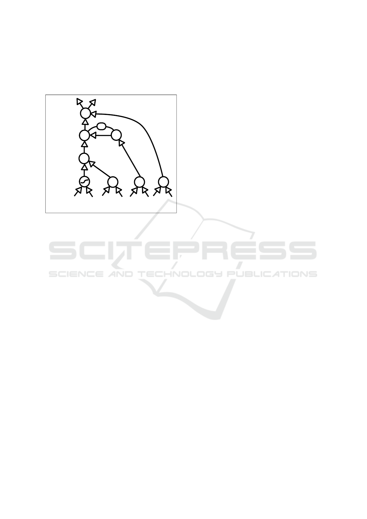
There is an activation function that is responsible for
determining when each of the gates should let the in-
formation flow or not (Hochreiter and Schmidhuber,
1997).
x
+
x
x x
x
x
Cell
Input
Output
Input
gate
Forget
gate
Output
gate
Figure 1: A memory cell from a LSTM neural network.
2.4 Related Works
Some recent papers relate works in the context of au-
tomatic lie detection. We have chosen four of the pa-
pers found in the literature. These works helped us to
specify a neural network basic-model for our experi-
ments and analyses.
The work of Liu (2004) (Liu, 2004) has a purpose
similar to the present work. It aims to detect voice
stress levels through pitch and jitter, performing the
implementation of Bayesian hypothesis testing with
Matlab. For this work, the best result obtained was
87% accuracy. However, it was only possible to
achieve this result with a dependent speaker, that is,
the model behaved this way only in the voice analysis
of a single person, and using the Pitch voice feature.
For the multi-speaker test (independent speaker), the
accuracy value drops to 70% using the Pitch charac-
teristic.
The work of Nurc¸in et al. (2017) (Nurc¸in et al.,
2017) aims to detect lies, which is performed by
studying and analyzing the dilation of the pupil of
the human eye, using a neural network with the back-
propagation algorithm. The neural network was im-
plemented and fed with the 60 preprocessed samples.
Networks with various amounts of hidden layers were
tested: 2, 7, 10, 20, and 50. The one with the best re-
sults was the 10 layer network. During training, all
sample images were correctly classified by the net-
work. With these results, it was found, although not
tested with new images, that it is possible to clas-
sify images of pupils according to their dilation ac-
curately.
Chow and Louie (2017) (Chow and Louie, 2017)
have the objective of detecting a person’s lie using
speech processing and natural language through au-
dio recorded from the subject. An LSTM neural net-
work was used to accomplish this goal. The final
recurrent neural network model used was a single-
level, one-way drop-out Long-Short Term Memory
(LSTM). The results with this type of implementa-
tion were around 61 % to 63 % accuracy. The voice
characteristic used for the analysis was the MFCC.
In the work of Dede et al. (2010) (Dede and Sa-
zli, 2010), the objective is to perform isolated speech
recognition, employing the use of neural networks,
where the recognition of digits 0 to 9 uttered by a
speaker is performed. The neural network used is
a recurrent Elman type. In the tests performed, the
speech recognition system developed in this project
recognized the digits very accurately, for Elman net-
works a hit rate of 99.35 % was reached, in PNN net-
works the hit frequency was 100 %, and the MLP net-
work reached 98.75 %. The results obtained in this
study were very satisfactory and determine that Arti-
ficial Neural Networks are an adequate and effective
way to perform speech recognition.
3 METHODS
The hypothetical/deductive method was adopted in
our research since the objective is to prove their sus-
tainability of the following supposition: “It is possible
to detect a lie by analyzing voice stress using a neural
network.”
A literature search was conducted to find works
about automatic lie detection through some analysis
of the human body to understand more about how
and what are the most common methods of lie detec-
tion. Then a neural network basic-model was speci-
fied. From the specified basic-model, the neural net-
work was implemented. The network implemented
in the search for the most useful parameters was an-
alyzed. Finally, the results obtained were evaluated
and discussed.
The present research starts from the study of
specific-domains of knowledge and concerning the
problem in question, that is still open, without a
definitive solution.
In the following subsections, it is presented the
data used during the experiments, the preprocessing
performed, the classification model and experiments
performed are formalized.
ICAART 2020 - 12th International Conference on Agents and Artificial Intelligence
744
3.1 Data
One of the crucial stages of this work is related to the
samples to build the corpus. Our experiments involve
the speech of people, so the corpus must contain la-
beled audio files related to the answers of subjects.
The first step to record the audio samples was to
create an interview model, in which one person asks a
question and the subject answer it. The aim is to cap-
ture the subject’s answer. A questionnaire was created
to be followed as an interview script, consisting of 11
questions. After each question asked to the subject,
he answers them, thus creating a dialogue. The inter-
view is conducted twice with each, the first time the
subject answers the questions telling lies, and the sec-
ond time the subject answers speaking the truth. So,
we have samples labeled as true or false (lie) answers.
The interview was conducted with 10 male subjects,
in the Brazilian Portuguese language, members of the
Applied Intelligence Laboratory (LIA) of the “Uni-
versidade do Vale do Itaja
´
ı”, and members of a group
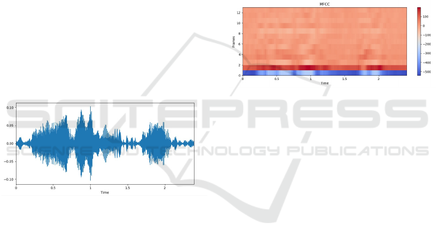
outside the university. Figure 2 shows the amplitude
of a person’s voice from an audio file of the corpus.
The x-axis represents time, and the y-axis represents
frequency amplitudes.
Figure 2: Graphical voice amplitude representation.
3.2 Preprocessing
During the preprocessing, it was used the software
Audacity, a free audio recording and editing software.
As each round of questions was recorded continu-
ously, without intervals, it was necessary to use Au-
dacity, to divide each interview into several separate
files, aiming only to contain the answers of the subject
because only these data compose the corpus. After
that, each answer was stored in a single file. Silence
present at the beginning and end of the files were re-
moved. Finally, the files are labeled as true or false
answers.
After completing the editing of all the interviews,
they resulted in a total of 220 audio files, 110 lying
answers, and 110 telling the truth, with a balanced
numerical proportion to represent each class of the
problem. Of the 220 files, 180 were assigned to be
used in network training, and the other 40 answers
were separated for classification tests. The files to
perform the classification tests were not used in neural
network training. The choice of the samples that was
used in the training and test occurred as follows: from
each interviewed, 9 files were randomly assigned to
be used in training, and 2 files designated for testing,
keeping the same proportion for all the subjects. The
duration of each audio file is variable. It can be 1 sec-
ond or even 7 seconds. Figure 3 shows a graph repre-
senting the MFCC spectrogram that corresponds to an
audio file extracted from the corpus, where the x-axis
indicates the time, the y-axis indicates the amount of
MFCC, and the colors represent the intensity of the
spectral density of energy present at each frequency
of the sound.
Figure 3: MFCC Espectrogram.
3.3 Input Processing and Feature
Extraction
The python language has a library for music and au-
dio analysis, called Librosa. In the first step of the al-
gorithm implementation, the library was used to load
the audio files from inside the corpus directory. The
audios were loaded by the library with a sample rate
of 22050 Hz, which is the number of samples per sec-
ond. After uploading all database files, the next step
is to extract the MFCC characteristics from each of
them.
For each uploaded file, another Librosa library
function is applied, which is a function responsible
for extracting the MFCC characteristics from them.
The amount of MFCC extracted in each audio file is
predefined as a parameter passed to the function, ini-
tially this value was set to 13, then to 20 and later to
40. Thus obtaining three different datasets results in
the time of extraction and allowing more significant
variation of the scenario in the training and testing of
the neural network. For each audio file, a data matrix
is generated, which is the size relative to the length
of the recorded audio, and the number of MFFC ex-
tracted.
As the extracted audio sequences vary in size ac-
cording to the length of time the recording has, it is
Novel Lie Speech Classification by using Voice Stress
745

not possible to infer these variable-length sequences
directly from the neural network. A sequence size
normalization technique called padding is used in this
project to solve this situation. The padding process
proceeds as follows when the MFCC audio sequences
are generated, it is verified which one has the largest
size, and based on it, all other smaller sequences are
remodeled to have the same size, but filling empty
spaces with the value 0. An auxiliary vector is cre-
ated, and it is assigned the actual size that each au-
dio sequence has. This is of great importance, as this
information is passed on to the neural network, and
then it will have a reference to how far it can pro-
cess each sequence, and what values it can disregard,
which in this case will be from the actual size, local
to the which padding was performed.
After extracting the voice characteristics of the
corpus, and normalizing them all, the next step is to
label the inputs, that is, to determine which class it be-
longs. At the moment each audio file has the extracted
MFCC characteristics, there is an auxiliary vector that
stores the information about which category that input
belongs to (being, 0 = Lie and 1 = Truth). The one-hot
encoding technique was used to transform this cate-
gorical data into numerical values. In this way, the
integer values representing classes 0 and 1 are trans-
formed into a vector in which the first position is for
the lie category, and the second position is for the
truth category. To say that a given audio input has
a category, place the value bit 1 at the position of the
vector representing that category, and the rest of the
positions must be filled with the value bit 0, always
considering the fact that each sample must belong to
only one class.
When the feature extraction, sequence normaliza-
tion, and class coding step is completed, the result is
a three-dimensional matrix with the MFCC character-
istics of the interviewees’ voice. Before starting train-
ing, this data is shuffled, resulting in the data set ready
to be inferred from the neural network, in which the
characteristics are analyzed, and the network training
is performed.
3.4 Classifier Model
The task of the neural network for this work is clas-
sification, and the type of learning employed in the
neural network is supervised. For this reason, there
is a training input dataset with related output. These
are the predefined categories for that data. During the
training, the model will be adjusted to map the inputs
to their corresponding outputs, finding patterns that
correspond to this association between the data and
the label.
The main processing core of the entire project is
defined as the prediction model, which essentially
consists of a learning algorithm and training data.
Within this prediction model, the neural network is
instantiated, and through a set of parameters is de-
fined the number of layers, the number of neurons per
layer, the calculation of weights and bias, and the ac-
tivation function. In the model, training data is in-
ferred, and the loss function, which is responsible for
performing each training iteration, calculates and ver-
ifies how close the network has come to mapping in-
puts according to correct outputs. With each error en-
countered, the learning algorithm will update and ad-
just the weights of neural network neurons to find the
best training results.
The loss function used in this work is “cross-
entropy” for “softmax”, which can be accessed using
a TensorFlow API (Application Programming Inter-
face) method. This type of loss function is most often
used to quantify the difference between two probabil-
ity distributions, in which an output vector represent-
ing the probability distribution is returned.
The activation function used in the neural net-
work of this work is “softmax”, which is very efficient
when the problem is classification of data.
To perform the training, with the optimization al-
gorithm Adam Optimizer was used, which is an algo-
rithm that can be used replacing the classic (relatively
slow) stochastic gradient descent procedure to update
the weights of the neural network in an iterative way,
from the training data.
The dimensions of the input layer of the neu-
ral network are variable to the size of the presented
dataset. It varies according to the size of the sample
batch, the number of MFCC per sample, and the size
of the sequences for each sample.
The number of nodes in the output layer is propor-
tional to the number of classes defined for the input
network samples, and the number of samples that are
inferred from the neural network. Thus, a probability
distribution is generated for the classes defined for the
network.
All prediction model hyperparameters are first as-
signed a value to start experiments. They are ad-
justable values and set before the start of network
training. The following parameters are defined: learn-
ing rate, the number of hidden layers, the number of
nodes per hidden layer; batch size; the number of it-
erations; and MFCC number per sequence. Figure
4 shows a diagram representing the prediction model
algorithm steps.
ICAART 2020 - 12th International Conference on Agents and Artificial Intelligence
746
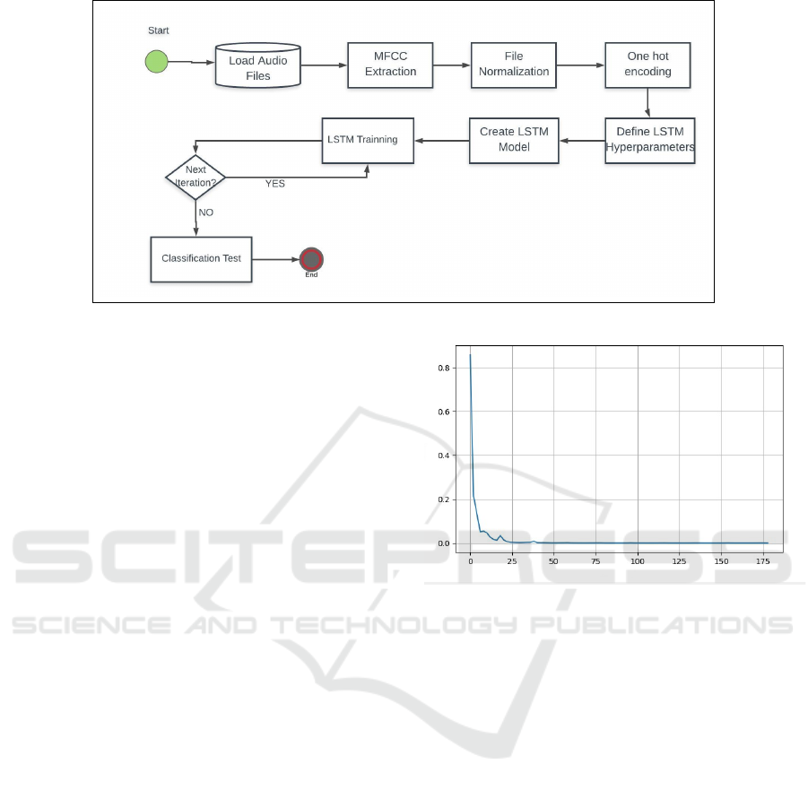
Figure 4: Fluxogram of Algorithm.
3.5 Experiments
After the parameter definition, the algorithm was ex-
ecuted. The neural network graph is initialized, and
the training step is started. At each time, the data
is inferred from the neural network prediction model,
and the process is repeated until the required number
of iterations is reached. At the end of each iteration,
the loss function is calculated, which will represent
how close that training step is to the desired results,
and as the result of the calculated error, the optimiza-
tion algorithm performs the adjustment of the network
weights and biases, search to decrease the error value,
and the algorithm proceeds to the next iteration of the
training.
When all training iterations are completed, the
prediction model receives the test samples, and then
the number of samples that have been correctly clas-
sified is calculated, thus obtaining the accuracy of this
model. Analyzing the accuracy result, the closer to 1
the value, the greater the number of samples that were
correctly classified; the closer to 0, the greater the
number of errors during the classification of the test
samples. Figure 5 shows a graph of the loss function
value according to the iteration number. It is possible
to see the value of the loss function approaching zero
when the number of iterations increases.
4 RESULTS
Only the most effective results were selected among
all sets of tested parameters and models. The results
have significance and precision above a chance. Ta-
ble 1 lists the prediction models with their respective
hyperparameters, and the accuracy reached by each
of them. It is necessary to define the hyperparam-
Figure 5: Loss Graph.
eters that are responsible for configuring the neural
network topology and the training process to perform
the training. The column “Model No.” that is present
in Table 1, is only to facilitate the identification of the
model when it is quoted later in the text.
Several parameter settings are combined to ensure
good performance in training and testing. The “Lay-
ers” column represents the number of hidden layers
of the neural network that are responsible for all input
data processing. The “Cells” column is the number
of LSTM cells in each hidden layer of the network,
each unit of cell performs the processing of a charac-
teristic, and directs its processing output to the next
layer. The column “No.MFCC” refers to the amount
of MFCCs characteristics present in each audio file of
the data set used in neural network training and test-
ing. Regarding “Batch”, the training dataset is made
up of a total of 180 entries with MFCC character-
istics, but this set of entries can be broken up into
smaller batches for training, which are called mini-
batches. Because the entries have been fragmented
into smaller batches, each iteration goes through only
one batch, and the training season will only be re-
alized when all the mini-batches in the set are fully
Novel Lie Speech Classification by using Voice Stress
747

run. “Iterations” corresponds to each training step
performed, which is completed when a batch is taken.
“Learn. Rate” refers to the size of the change made
by the learning algorithm in neural network weights.
Thus, the higher this value, the greater will be the
changes in neural network weights during training.
“Accuracy” is the percentage of correct classifications
in the test set that the neural network model obtained
after performing the training.
Model 1 presented an accuracy of 72.5% and was
the highest reached in this work. This model reached
a total of 29 samples correctly classified, 11 sam-
ples classified wrong, totaling the 40 tested samples.
Among these errors, 6 are false positives, and 5 are
false negatives.
Model number 2 brought very relevant results, as
described in Table 1 presented an accuracy of 70.0%.
This model reached a total of 28 correctly classified
samples, 12 wrong classified samples, totaling 40 test
samples. Of these errors, 5 are false positives, and 7
are false negatives.
Following Table 1, model number 3 presented an
accuracy of 67.5%. This model reached a total of 27
correctly classified samples, 13 wrong classified sam-
ples, totaling 40 test samples. Of these errors, 6 are
false positives, and 7 are false negatives.
The next model listed is number 4 which showed
an accuracy of 65.0% as described in Table 1. This
model reached a total of 26 correctly classified sam-
ples, 14 wrongly classified samples, totaling 40 test
samples. Of these errors, 5 are false positives, and 9
are false negatives.
Model number 5, as described in Table 1, pre-
sented an accuracy of 55.0%. Among all the models
mentioned, this was the one that reached the lowest
result. This model reached only a total of 22 correctly
classified samples, 18 wrongly classified samples, to-
taling 40 test samples. Of these errors, 9 are false
positives, and 9 are false negatives. This model is the
only one in the results presented, which has the value
of 40 of MFCC. For this parameter setting, despite
the low result, it was the model that brought the most
significant result.
It may be possible to perceive that there are simi-
larities in the parameters of each model. For the layer
quantity parameter, values were only between 3 and
4, and when using values smaller or larger than this,
we have noticed that there is no better result. The
number of cells in the hidden layers was between 200
and 300. Out of this range, there were no results with
any significance. The file batch size was defined on
all models with a value of 64, which brought stabil-
ity to the model when it was trained several times,
always producing equivalent and more stable results.
The number of iterations was between 100 and 180,
and it was observed that when the number of itera-
tions was higher than 200, it produced an overfitting
behavior in the model. This means that the model pre-
sented good classification results during training, but
for a set of new data, which is the data for testing, the
model demonstrates inefficiency. The learning rate
showed variable values according to each model. It
can be observed in a considerably high-value range,
varying from 0.001 to 0.01. One of the parameters
that greatly influenced the results was the number of
MFCCs, in which models defined with values of 13
and 20, proved to be much more effective in the re-
sults than the model that had 40 MFCC. The high-
est accuracy obtained by a model with 40 MFCC was
55.0%, which is an inaccurate result and does not rep-
resent that the model is an effective classifier.
5 CONCLUSIONS AND FINAL
REMARKS
The work-related in this paper aims to analyze an
LSTM performance when classifying a person’s voice
answer as reliable or not. For that, it was necessary
to verify which prediction models implemented led
the best results by checking its accuracy. By verify-
ing directly, the model that has the highest number of
correct ratings during the tests demonstrates the most
efficient in the results. In the final stage of this work,
the most relevant results were listed, and among them,
the one that showed the most prominence is a model
that reached an accuracy of 72.5%. That is, 72.5%
of the test samples were classified correctly. It is still
possible to state that there was a relevant statistical
significance since the model behaved above the level
of chance. For the context of this study, which is lie
detection through the analysis of voice answers, the
results obtained in this project can be considered rel-
evant, since there is no such result in the literature.
It can be observed that the obtained results are
close to other similar works. Similar work using sim-
ilar technology with the experiment performed in this
project is the work of (Chow and Louie, 2017), where
the purpose is to find patterns of lying in the voice
(through the MFCC) and in the sample interview tran-
scripts, using as a prediction model a recurrent LSTM
neural network. Following these specifications, the
best result obtained in the work of (Chow and Louie,
2017) is 63% of accuracy, slightly lower than that
achieved in this work. One detail is that to perform
the work of CHOW and LOUIE, was used a dataset
ready for the type of problem to be solved, and with
a large number of samples, which can significantly
ICAART 2020 - 12th International Conference on Agents and Artificial Intelligence
748

Table 1: Results of each tested basic-model and its accuracy.
N
o
Model Layers Cells N
o
MFCC Batch Iterations Learn. Rate Accuracy (%)
1 3 300 13 64 150 0.01 72.5
2 4 300 20 64 100 0.003 70.0
3 3 300 13 64 80 0.003 67.5
4 4 200 20 64 100 0.003 65.0
5 3 300 40 64 180 0.001 55.0
facilitate the elaboration of other steps of the work,
and significantly increase results according to data set
size.
Another work with similar purpose and that can
be used as a comparison parameter is that of (Liu,
2004), which aimed to detect stress levels in the voice,
through pitch and jitter, performing the implementa-
tion of Bayesian hypothesis with MatLab. The re-
sult of this work reached an accuracy of 87%; how-
ever, this result was only possible on test occasions
in which the trained classifier system was dependent
on the individual speaker, which corresponds to the
fact that the system was trained and tested only with
the voice of a single person. For tests performed in
which the system was trained with the voice of sev-
eral speakers, the best accuracy achieved was 70%,
which represents a value slightly lower than the re-
sult found in this work, which was 72.5%. It is note-
worthy that the (Liu, 2004) dataset was built by him-
self, through audio recordings that occurred during a
game, in which the participants’ goal was to lie to win.
Regarding the problems presented at the begin-
ning of this paper, the results suggest it is possible
to state that there is the possibility of detecting lies
through the speech of the individual using a neural
network. Since lie detection is an open problem, the
main contribution of this paper was to relate the stress
level of the voice as an inducer to detect lies. The use
of Deep Learning to perform this procedure, being un-
precedented, characterizes a contribution to the state-
of-the-art. As future works, we suggest the use of
more massive voice databases than used in this work,
including a diversity of accents and languages.
ACKNOWLEDGEMENTS
This work is partly supported by the “Universidade
do Vale do Itaja
´
ı” and “Universidade Federal de Santa
Catarina”.
REFERENCES
Cardoso, D. P. (2009). Identificac¸
˜
ao de locutor usando mod-
elos de misturas de gaussianas. Master’s thesis, Escola
Polit
´
ecnica, Universidade de S
˜
ao Paulo, S
˜
ao Paulo.
Childers, D. G., Skinner, D. P., and Kemerait, R. C. (1977).
The cepstrum: A guide to processing. Proceedings of
the IEEE, 65(10):1428–1443.
Chow, A. and Louie, J. (2017). Detecting lies via speech
patterns.
Council, N. R. (2003). The Polygraph and Lie Detection.
The National Academies Press, Washington, DC.
Damphousse, K. (2009). Voice stress analysis: Only 15
percent of lies about drug use detected in field test.
NIJ Journal, 259.
Dede, G. and Sazli, M. (2010). Speech recognition with
artificial neural networks. Digital Signal Processing,
20:763–768.
Hochreiter, S., Bengio, Y., Frasconi, P., and Schmidhuber, J.
(2001). Gradient flow in recurrent nets: the difficulty
of learning long-term dependencies. In Kremer, S. C.
and Kolen, J. F., editors, A Field Guide to Dynamical
Recurrent Neural Networks. IEEE Press.
Hochreiter, S. and Schmidhuber, J. (1997). Long short-term
memory. Neural computation, 9(8):1735–1780.
Kremer, R. L. and Gomes, M. L. d. C. (2014). A efici
ˆ
encia
do disfarce em vozes femininas: uma an
´
alise da
frequ
ˆ
encia fundamental. ReVel, 12(23):28–43.
Liu, X. F. (2004). Voice stress analysis: Detecion of decep-
tion. Master’s thesis, Department of Computer Sci-
ence – The University of Sheffield.
Nurc¸in, F., Imanov, E., Is¸ın, A., and Uzun Ozsahin, D.
(2017). Lie detection on pupil size by back propa-
gation neural network. Procedia Computer Science,
120:417–421.
Office of Technology Assessment’s (1983). Scientific valid-
ity of polygraph testing: a research review and evalu-
ation. Technical report, U.S. Congress.
Rao, K. R. and Yip, P. (1990). Discrete Cosine Trans-
form: Algorithms, Advantages, Applications. Aca-
demic Press Professional, Inc., San Diego, CA, USA.
Teixeira, J., Ferreira, D., and Carneiro, S. (2011). An
´
alise
ac
´
ustica vocal - determinac¸
˜
ao do jitter e shimmer para
diagn
´
ostico de patalogias da fala.
Tiwari, V. (2009). Mfcc and its applications in speaker
recognition. International Journal on Emerging Tech-
nologies.
Novel Lie Speech Classification by using Voice Stress
749
