Nash Equilibria in Multi-Agent Swarms

Carsten Hahn, Thomy Phan, Sebastian Feld, Christoph Roch, Fabian Ritz, Andreas Sedlmeier,

Thomas Gabor and Claudia Linnhoff-Popien

Mobile and Distributed Systems Group, LMU Munich, Munich, Germany

carsten.hahn, thomy.phan, sebastian.feld, christoph.roch, fabian.ritz, andreas.sedlmeier, thomas.gabor,

Keywords:

Multi-Agent Systems, Reinforcement Learning, Nash Equilibrium, Partial Observability, Scaling.

Abstract:

In various settings in nature or robotics, swarms offer various beneﬁts as a structure that can be joined easily

and locally but still offers more resilience or efﬁciency at performing certain tasks. When these beneﬁts are

rewarded accordingly, even purely self-interested Multi-Agent reinforcement learning systems will thus learn

to form swarms for each individual’s beneﬁt. In this work we show, however, that under certain conditions

swarms also pose Nash equilibria when interpreting the agents’ given task as multi-player game. We show

that these conditions can be achieved by altering the area size (while allowing individual action choices) in

a setting known from literature. We conclude that aside from offering valuable beneﬁts to rational agents,

swarms may also form due to pressuring deviants from swarming behavior into joining the swarm as is typical

for Nash equilibria in social dilemmas.

1 INTRODUCTION

Flocking behavior can be observed in many species

in nature. For example ﬁsh or birds coordinate their

actions in order to form a swarm. This yields ben-

eﬁts like: hydrodynamic efﬁciency, higher mating

chances, enhanced foraging success, enhanced preda-

tor detection, decreased probability of being caught

and overall reduced individual effort. In order to proﬁt

from such beneﬁts, swarming has also been trans-

ferred to technical systems featuring multiple robots

or drones (Brambilla et al., 2013; Christensen et al.,

2015). Swarms can be especially useful when they

allow to use smaller, simpler and effectively cheaper

robots and use the swarm to still allow for complex

behavior and error resilience (against communication

failures, bugs or external inﬂuences). However, since

swarms rely on the emergent behavior of a group of

individual agents, swarm behavior is often hard to

pre-program or even just predict (Pinciroli and Bel-

trame, 2016).

In this paper, we consider the issue of swarms con-

sisting of self-adaptive, learning agents and raise the

question under which conditions these agents tend to

form swarms purely out of self-interest. Here, mul-

tiple agents coming together within a swarm in the

ﬁrst place is not given or programmed but on its own

already an emergent behavior.

Ozg

uler and Yıldız

(

Ozg

uler and Yıldız, 2013) introduced a theoretical

model to examine how swarms form. They mod-

eled foraging swarm behavior as a non-cooperative N-

player game and have shown that the resulting swarms

pose a Nash equilibrium.

Hahn et al. (Hahn et al., 2019) have considered a

continuous predator-prey scenario where a swarm of

agents (resembling ﬁshes) aims to survive for as long

as possible in the presence of an enemy agent (resem-

bling a shark, e.g.). Under certain conditions, swarms

in such Multi-Agent system can emerge solely by

training (using reinforcement learning, e.g.) each

agent on the purely self-interested goal of securing

its own survival. It has been observed that the agents

learn to form clusters because the predator can be dis-

tracted by multiple agents in its vicinity, which in-

creases the survival chance of any individual. In their

work only the prey agents are actively trained while

the present predator follows a predeﬁned static heuris-

tic strategy. The prey agents are self-interested and

maximize solely their own reward (i.e., surviving as

long as possible). The group of agents is trained by

iteratively training only one of the prey agents and

copying its learned policy to all other homogeneous

agents.

The work of (Hahn et al., 2019) focuses mainly

on the examination of the resulting swarms and their

comparison to existing related swarm approaches

234

Hahn, C., Phan, T., Feld, S., Roch, C., Ritz, F., Sedlmeier, A., Gabor, T. and Linnhoff-Popien, C.

Nash Equilibria in Multi-Agent Swarms.

DOI: 10.5220/0008990802340241

In Proceedings of the 12th International Conference on Agents and Artiﬁcial Intelligence (ICAART 2020) - Volume 1, pages 234-241

ISBN: 978-989-758-395-7; ISSN: 2184-433X

(Reynolds, 1987; Morihiro et al., 2008). But they also

investigate origin and characteristics of the social be-

havior between prey agents and hint that the swarm

behavior of multiple self-interested agents trained us-

ing Multi-Agent reinforcement learning is linked to

Nash Equilibria.

We build on this foundation to further investigate

Nash equilibria in Multi-Agent swarms resulting from

Multi-Agent reinforcement learning. We adopt the

scenario of (Hahn et al., 2019) for our research and

further examine the conditions under which forming

a swarm pays off for each individual agent or un-

der which running individually is the superior strat-

egy. We show that the partial observable scenario

can be expanded and the learned policies can adapt

without any re-training. We relax the imposed crite-

ria on agent homogeneity, i.e., we allow each agent to

choose for itself if it wants to join a swarm or roam on

its own. We observe that this decision poses a social

dilemma as swarms only offer a beneﬁt at a certain

size. However, we also show that some swarm con-

ﬁgurations form Nash equilibria under certain condi-

tions, which means that even when swarming might

not be the strictly superior strategy in a certain situa-

tion, deviating from an already instituted is still worse

for a single agent.

2 FOUNDATIONS

2.1 Reinforcement Learning

Reinforcement Learning (RL) is a machine learning

paradigm which models an autonomous agent that

has to ﬁnd a decision strategy in order to solve a

task. The problem is typically formulated as Markov

Decision Process (MDP) (Howard, 1961; Puterman,

2014) which is deﬁned by a tuple M = hS, A, P , R i,

where S is a set of states, A is the set of actions,

P (s

t+1

, a

) is the transition probability function and

R (s

, a

) is the scalar reward function. We assume

that s

, s

t+1

∈ S , a

∈ A, r

= R (s

, a

), where s

t+1

reached after executing a

in s

at time step t. Π is the

policy space.

The goal is to ﬁnd a policy π : S → A with π ∈ Π,

which maximizes the expected (discounted) return G

at state s

for a horizon h:

h−1

∑

k=0

· R (s

t+k

, a

t+k

) (1)

where γ ∈ [0, 1] is the discount factor.

A policy π can be evaluated with a value function

, a

) = E

, a

], which is deﬁned by the ex-

pected return when executing a

at state s

and fol-

lowing π afterwards (Bellman, 1957; Howard, 1961).

π is optimal if Q

, a

) ≥ Q

, a

) for all s

∈ S ,

∈ A, and all policies π

∈ Π. The optimal value

function, which is the value function for any optimal

policy π

∗

, is denoted as Q

∗

and deﬁned by (Bellman,

1957):

∗

, a

) = r

+γ

∑

∈S

P(s

, a

)·max

∈A

∗

, a

)}

(2)

When Q

∗

is known, then π

∗

is deﬁned by π

∗

) =

argmax

∈A

∗

, a

)}.

Q-Learning is a popular RL algorithm to approx-

imate Q

∗

from experience samples (Watkins, 1989).

In the past few years, Q-Learning variants based on

deep learning, called Deep Q-Networks (DQN), have

been applied to high dimensional domains like video

games and Multi-Agent systems (Mnih et al., 2015;

Hausknecht and Stone, 2015; Leibo et al., 2017).

2.2 Game Theory and Multi-Agent

Reinforcement Learning

Multi-Agent Reinforcement Learning (MARL) prob-

lems can be formulated as stochastic game M =

hS , A, P , R , Z, O, ni, where hS ,A, are P equivalently

deﬁned as in MDPs. n is the number of agents,

A = A

× ... × A

the set of joint actions, Z is the set

of local observations, and O(s

, i) is the observation

function for agent i with 1 ≤ i ≤ n. R = R

× ... × R

is the joint reward function, with R

, a

t,i

) being the

individual reward of agent i.

In MARL, each agent i has to ﬁnd a local policy π

which is optimal w.r.t. the policies of the other agents.

If the other agents change their behavior then agent

i also need to adapt, since its previous policy might

have become suboptimal. The simplest approach to

MARL is to use single-agent RL algorithms like Q-

Learning and scale them up to multiple agents (Tan,

1993; Leibo et al., 2017). In homogeneous settings,

the policies can be shared by effectively learning only

one local policy π

and replicate the learned policy

to all agents. This can accelerate the learning pro-

cess as experience can be shared during training (Tan,

1993; Foerster et al., 2016). While many other ap-

proaches to MARL in games exist which incorporate

global information into the training process (Foerster

et al., 2016; Lowe et al., 2017; Foerster et al., 2018;

Rashid et al., 2018), we focus on the simple case of

applying single-agent RL to games with policy shar-

ing.

Nash Equilibria in Multi-Agent Swarms

235

2.3 Swarm Intelligence

One of the most common approaches for generating

artiﬁcial ﬂocking behavior is the so called “Boids”

approach proposed by (Reynolds, 1987). Reynolds

proposed three basic steering rules which only require

local knowledge of an individual about other individ-

uals within its view radius. The rules are:

• Alignment: Steer towards the average heading di-

rection of nearby individuals

• Cohesion: Steer towards the average position

(center of mass) of visible individuals

• Separation: Steer in order to keep a minimum

distance to nearby individuals (to avoid collisions

and crowding)

If each individual follows these rules, naturally ap-

pearing swarm formations can be observed. Imple-

menting the rules can be done by expressing them as

forces that act upon an individual. They can be ex-

tended in order to repel from an enemy or obstacles

respectively be attracted by food, for example.

Hahn et al. (Hahn et al., 2019) introduced SELF-

ish, a Multi-Agent system in which multiple homoge-

neous agents (independently from each other) try to

survive as long as possible while a predator is chasing

them. The predator might get distracted by multiple

preys in its vicinity. Hahn et al. showed that agents

trained using Multi-Agent reinforcement learning re-

alize to exploit this property by forming a swarm in

order to increase their survival chances. This swarm-

ing behavior is extensively examined and compared

to other swarming/ﬂocking algorithms (for example

the “Boids” approach). Furthermore (Hahn et al.,

2019) measured the survival time of the agents and

compared it to other policies, among others a hand

crafted policy called TurnAway. By following the

TurnAway strategy, agents turn in the opposite direc-

tion the predator and ﬂee without considering other

agents or obstacles. Hahn et al. ended their paper

with a hypothesis of Nash equilibria in Multi-Agent

swarms. This hypothesis will be picked up and ex-

tended in this work.

Ozg

uler and Yıldız (

Ozg

uler and Yıldız, 2013)

also investigated Nash equilibria in Multi-Agent

swarms. To do so, they modeled the foraging pro-

cess of multiple agents as a non-cooperative N-player

game. They assumed that each agent wants to min-

imize its individual total effort in a time interval by

controlling its velocity. By establishing a nonlin-

ear differential equation in terms of positions of the

agents and solving this equation they show that the

game has a Nash equilibrium.

2.4 Nash Equilibria

Game theory considers strategic interactions within a

group of individuals. In doing so, the actions of each

individual affect the outcome and the individuals are

aware of this fact. In addition, the participating indi-

viduals are considered rational. This means, that they

have clearly deﬁned goals within the possible out-

comes of the interactions and that they implement the

best available strategy to pursue their goals. Usually,

the rules of the game and rationality are well known.

Basically, two different forms of representation

exist: the normal form is used when the players

choose one strategy without knowing the others’

choices. The extensive form is used when some play-

ers know what other players have done while play-

ing. In many settings, no communication between the

players is possible or desired, which is why in the

following only the normal form game (also: strate-

gic form game) is described. A normal form game

G = (N, {A

}

i∈N

, {u

}

i∈N

) consists of a set of play-

ers N, a set of actions with A

for each player i and a

payoff function u

: A → R for each player i. The ac-

tion proﬁle a = (a

, ..., a

) is a collection of actions,

one for each player, also called strategy proﬁle. a

−i

is a strategy proﬁle without the action of player i. All

possible collections of actions are also called space of

action proﬁles A = (a

, ..., a

) : a

∈ A

, i = 1, ..., n.

A Nash Equilibrium (NE) is a strategy proﬁle so

that each strategy is a best response to all other strate-

gies. A best response is the reaction to an action that

maximizes the payoff.

Expressed in formal terms, a result a

∗

, ..., a

∗

) is a Nash Equilibrium, if for every player i

the following holds: u

∗

, a

∗

−i

) ≥ u

, a

∗

−i

) ∀a

∈ A

The most interesting feature about NEs is that they

are self-assertive: no player has an incentive to devi-

ate unilaterally.

Regarding the swarm environment in this pa-

per, the self interested agents correspond to the

non-cooperative players of a normal form game.

SELFish

DQN

and TurnAway, which will be explained

in the Section 3 match to the possible set of actions,

a player, respectively agent, can choose from. The re-

ward of a agent, which correlates to the survival time

of an individual corresponds to the payoff of a certain

strategy proﬁle. With deﬁning such a swarm environ-

ment as a normal form game it is possible to ﬁnd NEs

with a common Nash solver. In this work the popular

Gambit Solver was used (McKelvey et al., 2016).

ICAART 2020 - 12th International Conference on Agents and Artiﬁcial Intelligence

236

2.5 Social Dilemmas in Multi-Agent

Systems

In many Multi-Agent Systems, agents need to co-

operate in order to maximize their own utilities.

In (de Cote et al., 2006), the authors analyze Multi-

Agent social dilemmas in which RL algorithms are

confronted with Nash Equilibria forming a rational

optimal solution on the short term but not being op-

timal in repeated interaction. They propose heuris-

tic principles to improve cooperation and overcome

such one-shot Nash Equilibrium strategies. However,

their experiments are limited to a prisoner’s dilemma

scenario with three agents and four actions. More

recently, (Leibo et al., 2017) demonstrated that the

learned behavior of agents in Multi-Agent systems

changes as a function of environmental factors. They

experimentally show how conﬂicts can emerge from

competition over shared resources and how the se-

quential nature of real world social dilemmas affects

cooperation. While their environments’ complexity is

comparable to this paper’s, their experiments are lim-

ited to two agents. Nevertheless, the Nash Equilibria

suspected in (Hahn et al., 2019) and further examined

in this paper shares many characteristics with the se-

quential social dilemmas introduced in (Leibo et al.,

2017). The swarming behavior learned is a strategy

spanning over multiple actions and is experimentally

shown to not be the optimal strategy for the collective

of agents. But as swarming behavior clearly requires

some form of coordination, the analysis of whether or

not swarming may be considered a defect in the sense

of (Leibo et al., 2017) is left open for further analysis.

3 EXPERIMENTAL SETUP

3.1 SELFish Environment

We use the same environment as (Hahn et al., 2019)

and extend their experiments. The agents can roam

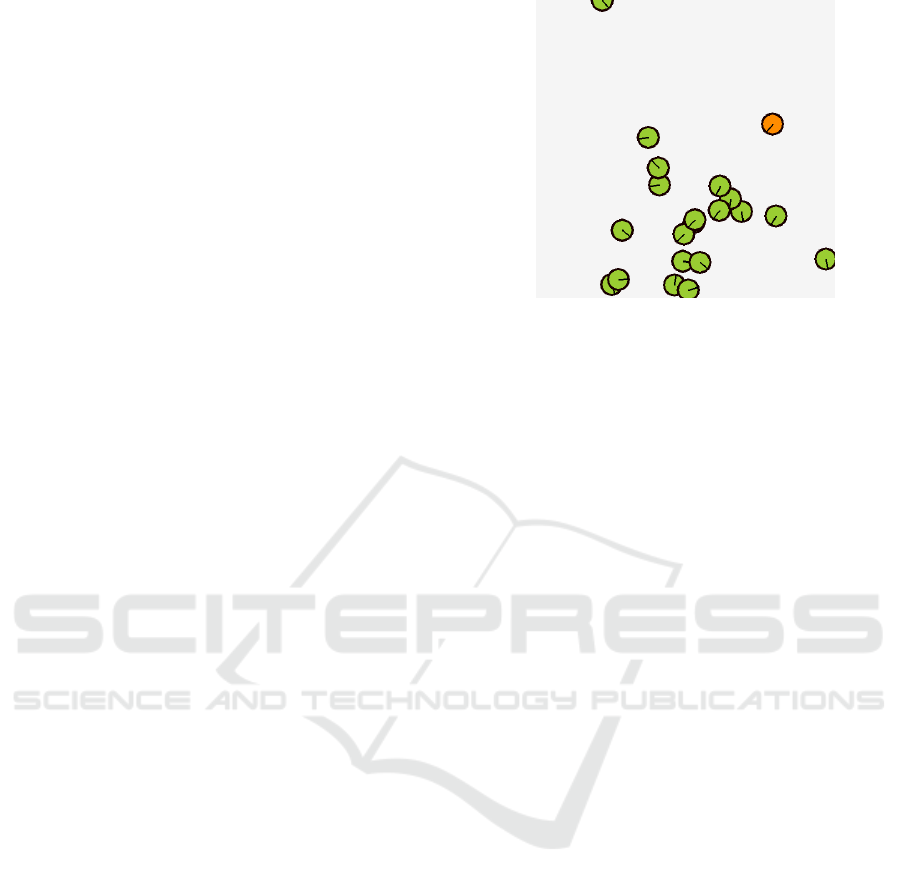
freely in a two-dimensional area (see Figure 1). The

area wraps around at the edges, meaning an agent that

leaves it on the right side will immediately re-enter it

from the left (same with top and bottom). Aside with

the trained agents the environment is inhabited by a

predator which pursues a predeﬁned static policy. The

predator can sense prey agents within a certain radius

and chooses one randomly as target (and keeps this

target for a certain time). This means that the preda-

tor might be distracted by multiple agents in its prox-

imity, which implies that it might be beneﬁcial for an

agent to be close to others, thus modeling one of the

Figure 1: Example visualization of the environment show-

ing the agents in green and the predator in orange. The black

line shows the movement direction of the respective agent.

established beneﬁts of joining a swarm. Both the prey

agents and the predator are embodied as circles with

a certain radius and a variable orientation (see Fig-

ure 1). A prey agent is considered caught when it

collides with the predator. It is then immediately re-

spawned in the area. The predator and the prey usu-

ally move at the same speed to encourage situations

in which a prey agent can escape from the predator

when it gets distracted. However, because of the torus

property of the area, this would allow a prey agent to

simply turn in the opposite direction of the predator

and move away without the possibility of the predator

ever catching up. That is why the predator increases

its speed every 80 steps over a duration of 20 steps.

The objective that is learned by the prey agents is

to survive as long as possible. This is reinforced with

a reward of +1 for each step survived and -1000 for

colliding with the predator. As soon as the learning

agent collides with the predator, the episode ends and

its knowledge is copied to all other agents.

As all agents move at a constant speed, the only

decision an agent has to make every step, is the

degree the agent wants to turn before it is moved

a certain unit in that direction. For DQN the ac-

tion space comprises of ﬁve discrete degree values

{−90

◦

, −45

◦

, 0

◦

, +45

◦

, +90

◦

3.2 State Encoding

The state of the environment is only partially observ-

able for an agent. This facilitates the scalability of

the approach and represents autonomous agents or bi-

ological individuals in reality as it is unlikely that an

individual can sense the whole state of any physical

environment/world. It is also in accordance with other

related swarming algorithms like (Reynolds, 1987)

where an agent only considers a local neighborhood

Nash Equilibria in Multi-Agent Swarms

237

of other agents and adjusts its direction according to

rules of cohesion, alignment and separation

In SELFish (Hahn et al., 2019), every agent can at

most observe n other entities (i.e., other prey agents

or the predator) in its vicinity. As observation, ev-

ery agent a receives for all other agents e

, i ∈ [1, n],

within its observation the distance between a and e

the angle a would have to turn in order to face in the

direction of e

and the absolute orientation of e

space. The angle an agent has to turn in order to face

to another observed entity is pre-calculated in degrees

in the range of (−180

◦

, 180

◦

]. The absolute orienta-

tion of an entity in space is measured in degrees in

the range of [0

◦

, 360

◦

). 0

◦

corresponds to facing east-

wards, measuring the angle counter-clockwise.

Every agent receives the previously explained

measurements as observation for the predator, itself

and for a certain number of n neighboring agents, in

which the n neighbors are ordered by their distance.

The measurements are ﬂattened into a vector before

they are handed to the agents. Furthermore the dis-

tance is divided by the area width and the direction

and orientation are normalized to the interval [0, 1].

3.3 Training

Training is performed using the Keras-RL (Plap-

pert, 2016) implementation of DQN. As DQN is in-

tended for single agent use, the training of the multi-

ple homogeneous agents is executed as proposed by

(Egorov, 2016): Only one agent is actually trained

and its policy is copied to the others after the end of

an episode. An episode ends if the learning agent is

caught by the predator or after 10, 000 steps were ex-

ecuted.

During the training the edge lengths of the area

always are 40 by 40 pixels. However, the agents as

well as the predator can take every real valued po-

sition in [0, 40] × [0, 40]. The agents and the preda-

tor have the size of a circle with radius 1, meaning a

collision (catch) occurs at a distance below 2. Please

note that no other collisions are considered (between

agents and other agents or agents and walls). Also

there are no obstacles in the area. During training

there are 10 agents in the environment.

In order to assess the quality of a training run, the

cumulative reward of the learning agent is measured.

According to the reward structure this essentially cor-

responds with the number of time steps the learning

agent survived.

Reproduced from (Hahn et al., 2019), the results

of training showed swarming behavior of the agents

in order to increase their survival chances, although

only 10 agents were present during training.

4 SCALING OF PARTIALLY

OBSERVABLE SCENARIOS

Because of the partial observability and the normal-

ization of the observation the learned policy of the

case with 10 agents can also be used in scenarios with

other parameters in regard to the number of agents

present or the size of the available area. This interre-

lationship will be further investigated in the following

section.

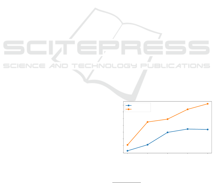
Figure 2 shows the average episode length, which

essentially corresponds to the average survival time of

a certain agent (i.e., the learning agent). An episode

ends if the learning agent is caught by the predator

or 10, 000 steps were made. As the learning agent

receives a +1 for every step and −1000 for being

caught, it is encouraged to survive as long as pos-

sible to maximize its accumulated reward. For the

static strategy of turning 180

◦

away from the preda-

tor without minding other agents (i.e., TurnAway) this

means that a certain agent is caught in order for an

episode to end.

. In Figure 2 the number of agents

is varied while the size of the area remains the same

(40×40 pixels). Please note that although the number

of agents is varied, the policy of SELFish

DQN

, which

was learned with 10 agents in the environment, stays

the same. One can see that the performance of the

policy, despite the fact that the environment settings

are modiﬁed, does not collapse. The increase of the

average episode length for higher number of agents

comes from the circumstance that, with more agents

in the environment, the probability decreases that any

particular agent is caught. The measurements for Tur-

nAway are given for comparison. Nevertheless, Fig-

ure 2 shows that TurnAway performs better w.r.t. the

20 40 60 80 100

Number of agents

1000

1500

2000

2500

3000

3500

4000

4500

Avg. episode lenght

SELFish

DQN

TurnAway

Figure 2: Average episode length (survival time) of the

learning agent in accordance with (Hahn et al., 2019). The

policy SELFish

DQN

was trained with 10 agents on 40 × 40

pixels and it then used for larger numbers of agents.

For a short video showing an example of the policies

SELFish

DQN

and TurnAway please refer to https://youtu.

be/nYKamj9qjFM

ICAART 2020 - 12th International Conference on Agents and Artiﬁcial Intelligence

238

average episode length or the survival time of a partic-

ular agent, respectively. This raises the question, why

this policy was not found by reinforcement learning,

which will be further examined in the following sec-

tion.

5 NASH EQUILIBRIA IN

SWARMS

As previously mentioned, 10 homogeneous agents

were trained on a 40 × 40 pixel area, while only one

agent was actually trained using reinforcement learn-

ing and its policy was copied to all other agents after

each episode. An episode ended if the learning agent

was caught by the predator (i.e. collided with it) or

10, 000 steps were executed. The reward was struc-

tured in such a way that the learning agent was en-

couraged to stay alive as possible. The predator has

the property that it might get distracted by multiple

prey agents in its proximity. That is why the agents

learned to form swarms in order to increase their sur-

vival chances. Another strategy in which the agent

always turned in the opposite direction of the preda-

tor and ﬂed without minding other agents was imple-

mented for comparison (TurnAway). Figure 2 showed

that the policy learned with 10 agents on a 40 × 40

pixel area can be used in settings with more agents

without breaking. But furthermore it showed that the

static policy of turning away performs better than the

learned policy in terms of survival time.

To further investigate this phenomenon we carry

out an experiment in which agents pursuing both poli-

cies (learned and static) are present. The results are

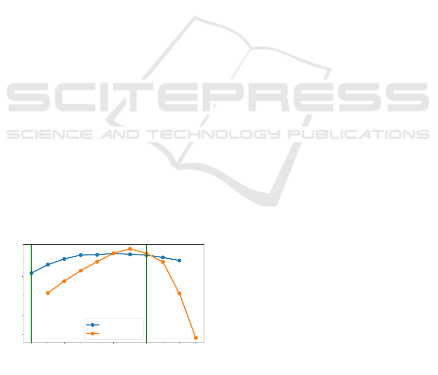
shown in Figure 3. Figure 3 shows a setup where

in an area of 40 × 40 pixels 10 agents are present.

These agents either use the learned SELFish

DQN

pol-

icy (trained with 10 homogeneous agents on 40 × 40

(0, 10)

(1, 9)

(2, 8)

(3, 7)

(4, 6)

(5, 5)

(6, 4)

(7, 3)

(8, 2)

(9, 1)

(10, 0)

(Number of TurnAway Agents, Number of SELFish

DQN

Agents)

200

300

400

500

600

Avg. survival time of an individual

SELFish

DQN

TurnAway

Figure 3: Performance of SELFish

DQN

(trained with 10

agents on 40×40 pixel) versus TurnAway on a 40×40 pixel

area. Nash equilibria marked with a green line.

pixel) or the static TurnAway policy. The agents

following SELFish

DQN

tend to form swarms as they

learned that this might increase their survival chances

(given the property of a distractible predator) while

TurnAway-agent do not care about others (except for

the predator). The abscissa illustrate the mixing pro-

portion of the agents with their particular type. For

example, the entry (6, 4) on the abscissa means that

there are 6 agents executing TurnAway and 4 agents

executing SELFish

DQN

in the setting. On the ordi-

nate the survival time (in steps) of individuals fol-

lowing either SELFish

DQN

or TurnAway is indicated

(averaged over individuals inside each policy type).

The experiment was carried out over 10 runs (with

different seeds), each with 10 episodes which lasted

100, 000 steps (with no other stopping criteria). This

resulted in thousand of caught agents in both pol-

icy groups whose survival time was then averaged.

Caught agents respawned at the most dense spot of the

swarm (determined with Kernel Density Estimation

(Phillips et al., 2006; Hahn et al., 2019)). This was

done because moving away from the swarm respec-

tively ignoring the action of other agents was of par-

ticular interest for this experiment and the swarm be-

havior should not be disturbed by respawning agents.

The experiment reveals multiple interesting in-

sights:

1. The performance of SELFish

DQN

w.r.t. the sur-

vival time in the setting it was actually trained on

is better than TurnAway. This means that the us-

age of a policy obtained in a partially observable

model in a setting with other parameters is possi-

ble but might not result in consistent performance

with the trained setting (cf. Figure 2).

2. Flocking behavior resulting from reinforcement

learning in this setting (multiple homogeneous

agents evading/distracting a predator) is a Nash

equilibrium (green line at (0, 10) in Figure 3).

This means that if there are 10 agents per-

forming SELFish

DQN

with a tendency to swarm-

ing/grouping (and zero performing TurnAway),

then no agent has an incentive to deviate from

this policy of “swarming” while all others keep

their strategy. We can see that moving out of the

swarm and ignoring the others (like TurnAway)

leads the agent onto the free space, where it is an

easy prey for the predator. We also conﬁrmed this

intuition by calculating the Nash equilibria with

the Gambit software tools for game theory (McK-

elvey et al., 2016). This was done by consid-

ering the average survival time of an agent pur-

suing a certain strategy as payoff in a normal-

form game. This means, for example, that if 9

agents perform SELFish

DQN

, the payoff of ev-

Nash Equilibria in Multi-Agent Swarms

239

ery agent following this strategy is 561 while the

one agent performing TurnAway has a payoff of

415. Gambit also revealed a less obvious Nash

equilibrium at (7, 3). At this point an agent per-

forming TurnAway (payoff 619) has no incentive

to switch its strategy to SELFish

DQN

(payoff 614

of SELFish

DQN

at point (6, 4). In addition, an

agent performing SELFish

DQN

(payoff 610) has

no incentive to switch to TurnAway (payoff 574

at (8, 2)) while the other agents keep their strat-

egy (see Table 1).

3. Policies in Multi-Agent scenarios produced with

DQN and the method proposed by (Egorov, 2016)

can only take the outer points (0, 10) and (10, 0)

as all agents perform the same policy. In the ex-

ample of an area size of 40 × 40 pixels, (0, 10) is

surely better while a ratio of (6, 4) is the best mix-

ture of both strategies (although) still not the best

performance achievable in this setting.

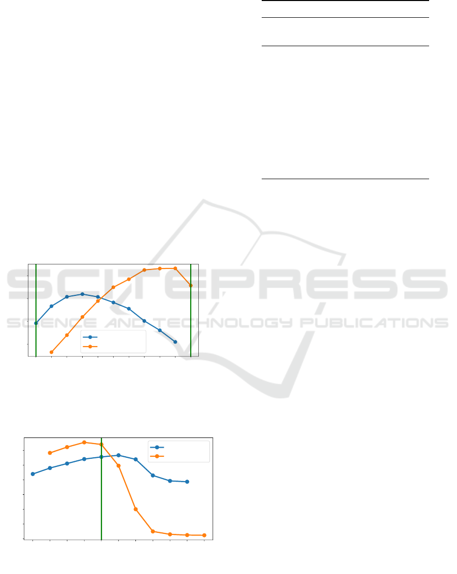
To further substantiate our results, we repeat this

experiment in area sizes of 80 ×80 and 20×20 pixels.

The results can be seen in Figure 4 and 5. They show

that the results vary for different area sizes, like pure

(0, 10)

(1, 9)

(2, 8)

(3, 7)

(4, 6)

(5, 5)

(6, 4)

(7, 3)

(8, 2)

(9, 1)

(10, 0)

(Number of TurnAway Agents, Number of SELFish

DQN

Agents)

1000

1200

1400

1600

Avg. survival time of an individual

SELFish

DQN

TurnAway

Figure 4: Performance of SELFish

DQN

(trained with 10

agents on 40×40 pixel) versus TurnAway on a 80×80 pixel

area. Nash equilibria marked with a green line.

(0, 10)

(1, 9)

(2, 8)

(3, 7)

(4, 6)

(5, 5)

(6, 4)

(7, 3)

(8, 2)

(9, 1)

(10, 0)

(Number of TurnAway Agents, Number of SELFish

DQN

Agents)

100

125

150

Avg. survival time of an individual

SELFish

DQN

TurnAway

Figure 5: Performance of SELFish

DQN

(trained with 10

agents on 40×40 pixel) versus TurnAway on a 20×20 pixel

area. Nash equilibria marked with a green line.

Table 1: Survival time/payoff of 10 agents with different

policies in an area of 40 × 40 pixels.

Number of agents Survival time

Turn SELFish Turn SELFish

Away

DQN

Away

DQN

0 10 nan 517

1 9 415 561

2 8 476 590

3 7 530 611

4 6 576 612

5 5 620 619

6 4 642 614

7 3 619 610

8 2 575 598

9 1 412 582

10 0 183 nan

TurnAway clearly outperforming pure SELFish

DQN

in the 80 × 80 pixel case and different Nash equilibria

like (4, 6) in the 20 × 20 pixel case.

6 CONCLUSION

In this paper we further examine the experimental

setup of (Hahn et al., 2019). Hahn et al. trained mul-

tiple homogeneous agents to evade a predator for as

long as possible. The predator in that setting follows

a static pre-deﬁned policy and can be distracted by

multiple possible preys in its vicinity. This modelled

one of the beneﬁts of forming a swarm and the agents

learned to exploit this circumstance accordingly.

Expanding this setup, we showed that policies ob-

tained through reinforcement learning in partially ob-

servable scenarios can be used in other settings with-

out a collapse of the performance, although consistent

performance (compared to the setting the policy was

actually trained on) cannot be guaranteed. Further-

more we showed that the swarm resulting from Multi-

Agent reinforcement learning in a predator/prey sce-

nario has a Nash equilibrium, i.e., that there are sce-

narios were speciﬁc swarm conﬁgurations are stable

(assuming rational agents) but still suboptimal. We

analyzed this effect in dependance of the area size.

We concluded swarming or not swarming can be for-

mulated as a social dilemma in some settings.

This sheds some light on the reasons why swarms

emerge. The introduction started by listing beneﬁts

observed from biological swarms. The presented re-

search, however, might list another reason for the for-

mation of swarms: social pressure. The existence

of a swarm of substantial size may actively impede

ICAART 2020 - 12th International Conference on Agents and Artiﬁcial Intelligence

240

the survival of non-swarming individuals, thus urging

them to join the swarm even when it is suboptimal

to all individuals’ survival. Note that this affects ra-

tional agents, i.e., swarm participants that act locally

optimal at every single one of their decisions.

Interestingly, the phenomenon of pressure aris-

ing from lack of communication and control struc-

tures has been observed in natural evolution as

well (Dawkins, 1976). Thus, swarms can (un-

der certain conditions) also be interpreted as self-

perpetuating, which means that they should be han-

dled with additional care when employing them

in practical applications. Self-perpetuating swarms

might introduce additional targets for emergent be-

havior that affect the system designer’s intended pur-

pose. It is up to future research to examine the inter-

play between using such emergent behavior and con-

trolling it to employ useful swarm applications.

REFERENCES

Bellman, R. (1957). Dynamic Programming. Princeton

University Press, Princeton, NJ, USA, 1 edition.

Brambilla, M., Ferrante, E., Birattari, M., and Dorigo, M.

(2013). Swarm robotics: a review from the swarm

engineering perspective. Swarm Intelligence, 7(1):1–

41.

Christensen, A. L., Oliveira, S., Postolache, O., De Oliveira,

M. J., Sargento, S., Santana, P., Nunes, L., Velez, F. J.,

Sebasti

ao, P., Costa, V., et al. (2015). Design of com-

munication and control for swarms of aquatic surface

drones. In ICAART (2), pages 548–555.

Dawkins, R. (1976). The Selﬁsh Gene. Oxford University

Press, Oxford, UK.

de Cote, E. M., Lazaric, A., and Restelli, M. (2006). Learn-

ing to cooperate in multi-agent social dilemmas. In

Proceedings of the Fifth International Joint Confer-

ence on Autonomous Agents and Multiagent Systems,

AAMAS ’06, pages 783–785, New York, NY, USA.

ACM.

Egorov, M. (2016). Multi-agent deep reinforcement learn-

ing. CS231n: Convolutional Neural Networks for Vi-

sual Recognition.

Foerster, J., Assael, I. A., de Freitas, N., and Whiteson, S.

(2016). Learning to communicate with deep multi-

agent reinforcement learning. In Advances in Neural

Information Processing Systems, pages 2137–2145.

Foerster, J. N., Farquhar, G., Afouras, T., Nardelli, N., and

Whiteson, S. (2018). Counterfactual multi-agent pol-

icy gradients. In Thirty-Second AAAI Conference on

Artiﬁcial Intelligence.

Hahn, C., Phan, T., Gabor, T., Belzner, L., and Linnhoff-

Popien, C. (2019). Emergent escape-based ﬂock-

ing behavior using multi-agent reinforcement learn-

ing. The 2019 Conference on Artiﬁcial Life, (31):598–

605.

Hausknecht, M. and Stone, P. (2015). Deep recurrent q-

learning for partially observable mdps. In 2015 AAAI

Fall Symposium Series.

Howard, R. A. (1961). Dynamic Programming and Markov

Processes. The MIT Press.

Leibo, J. Z., Zambaldi, V., Lanctot, M., Marecki, J., and

Graepel, T. (2017). Multi-agent reinforcement learn-

ing in sequential social dilemmas. In Proceedings of

the 16th Conference on Autonomous Agents and Mul-

tiAgent Systems, pages 464–473. International Foun-

dation for Autonomous Agents and Multiagent Sys-

tems.

Lowe, R., Wu, Y., Tamar, A., Harb, J., Abbeel, O. P.,

and Mordatch, I. (2017). Multi-agent actor-critic

for mixed cooperative-competitive environments. In

Advances in Neural Information Processing Systems,

pages 6379–6390.

McKelvey, R. D., McLennan, A. M., and Turocy, T. L.

(2016). Gambit: Software tools for game theory.

Mnih, V., Kavukcuoglu, K., Silver, D., Rusu, A. A., Veness,

J., Bellemare, M. G., Graves, A., Riedmiller, M., Fid-

jeland, A. K., Ostrovski, G., et al. (2015). Human-

level control through deep reinforcement learning.

Nature, 518(7540):529–533.

Morihiro, K., Nishimura, H., Isokawa, T., and Matsui,

N. (2008). Learning grouping and anti-predator be-

haviors for multi-agent systems. In Int’l Conf. on

Knowledge-Based and Intelligent Information and

Engineering Systems. Springer.

Ozg

uler, A. B. and Yıldız, A. (2013). Foraging swarms as

nash equilibria of dynamic games. IEEE transactions

on cybernetics, 44(6):979–987.

Phillips, S. J., Anderson, R. P., and Schapire, R. E. (2006).

Maximum entropy modeling of species geographic

distributions. Ecological modelling, 190(3-4).

Pinciroli, C. and Beltrame, G. (2016). Swarm-oriented pro-

gramming of distributed robot networks. Computer,

49(12):32–41.

Plappert, M. (2016). keras-rl. https://github.com/keras-

rl/keras-rl.

Puterman, M. L. (2014). Markov decision processes: dis-

crete stochastic dynamic programming. John Wiley &

Sons.

Rashid, T., Samvelyan, M., Witt, C. S., Farquhar, G., Foer-

ster, J., and Whiteson, S. (2018). Qmix: Monotonic

value function factorisation for deep multi-agent rein-

forcement learning. In International Conference on

Machine Learning, pages 4292–4301.

Reynolds, C. W. (1987). Flocks, herds and schools: A dis-

tributed behavioral model. In ACM SIGGRAPH com-

puter graphics, volume 21. ACM.

Tan, M. (1993). Multi-agent reinforcement learning: in-

dependent versus cooperative agents. In Proceed-

ings of the Tenth International Conference on Interna-

tional Conference on Machine Learning, pages 330–

337. Morgan Kaufmann Publishers Inc.

Watkins, C. J. C. H. (1989). Learning from Delayed Re-

wards. PhD thesis, King’s College, Cambridge, UK.

Nash Equilibria in Multi-Agent Swarms

241