Simulated Annealing Approach for the Vehicle Routing Problem with
Synchronized Visits
Seddik Hadjadj and Hamamache Kheddouci
Laboratoire d’Informatique en Image et Syst
`
emes d’Information, Villeurbanne, France
Keywords:
Vehicle Routing Problem, Simulated Annealing, Temporal Precedence Constraint, Synchronized Visits.
Abstract:
In this paper, we consider a vehicle routing problem in which customers have to be visited by two different
vehicles in a certain order. The first vehicle has to visit n customers to pickup or deliver empty containers, while
the second has to deliver ready-mixed concrete by pouring it into the previously delivered containers. This
problem is a vehicle routing problem (VRP) variant involving synchronized visits and temporal precedence
constraints.
We propose an ILP formulation and a simulated annealing algorithm to minimize the total travel times of both
vehicles, and we provide experiments that show very satisfying results.
1 INTRODUCTION
This work is carried out in collaboration with a com-
pany which is specialized in the sale of ready-mixed
concrete.
Today, a ready-mixed concrete order requires nec-
essarily the mobilization of one or more mixer trucks,
even when dealing with very small quantities of con-
crete. However, such type of truck is cumbersome,
expensive, and disproportionate in some cases, espe-
cially when delivering small quantities of concrete.
Therefore, the company proposes a new delivery
method to deal more effectively with such orders. The
idea is to share a single mixer truck by several cus-
tomers with small quantities (≤ 2000 liters), which
implies organizing optimized mixer truck tours.
On the other hand, to ensure the profitability of
these truck tours, waiting times at each customer’s lo-
cation have to be reduced. Today, a mixer truck has
to wait until the concrete is poured on site to leave a
customer’s location, and this causes a huge waste of
time. A solution to this problem is to pour the con-
crete from the truck into special containers instead of
pouring it directly on site which is more difficult and
takes more time. The truck can then leave faster, and
the customer can use the concrete in the containers all
day long. Waiting times are then drastically reduced.
However, since the containers which are supposed
to contain the concrete are special, they also must be
delivered to the customer. This implies dealing with
another vehicle tour to deliver the containers and pick
them up after they have been used.
In brief, this new method is a three-step process:
1. A vehicle delivers a number of empty containers
to the customer;
2. Thereafter, a mixer truck delivers a certain quan-
tity of ready-mixed concrete by pouring it into the
containers delivered;
3. The next day, the vehicle returns to the customer
to pick up the containers after they have been
used.
To ensure the profitability of this method, the com-
pany needs a decision support system that can gen-
erate two efficient and synchronized vehicle tours: a
pickup & delivery tour for the containers, and a mixer
truck tour to deliver the concrete, knowing that each
customer has to receive the containers before the con-
crete.
This problem is a vehicle routing problem vari-
ant involving combined vehicle tours and temporal
precedence constraints, it is then obviously NP-Hard
(Lenstra and Kan, 1981).
Despite the fact that synchronized vehicle tours
have several real world applications, there are, to the
best of our knowledge, only few works dealing with
such problems. Among these works, (Bredstr
¨
om and
R
¨
onnqvist, 2008) presented the “combined vehicle
routing and scheduling problem with time windows
and additional temporal constraint”. Some real world
problems have been presented, and a mathematical
Hadjadj, S. and Kheddouci, H.
Simulated Annealing Approach for the Vehicle Routing Problem with Synchronized Visits.
DOI: 10.5220/0008990302970303
In Proceedings of the 9th International Conference on Operations Research and Enterprise Systems (ICORES 2020), pages 297-303
ISBN: 978-989-758-396-4; ISSN: 2184-4372
Copyright
c
 2022 by SCITEPRESS – Science and Technology Publications, Lda. All rights reserved
297

programming model has been proposed. A heuris-
tic solution has also been studied to deal with real
world instances considering three different objective
functions: minimizing the total travel times, maxi-
mizing the sum of preference (a customer can prefer
being visited by a specific vehicle), and optimizing
the workload balance.
(Dohn et al., 2011) studied the vehicle routing
problem with time windows and temporal Depen-
dencies (VRPTWTD). Some specific constraints have
been considered like the minimum / maximum gap
between the starting time and the ending time of vis-
its and a branch and cut and price algorithm was pro-
posed to minimize the total travel cost.
Overall, most of papers dealing with vehicle rout-
ing problems with temporal precedence constraints
consider exact methods to solve those problems. Only
few works attempted to solve such problems with
heuristics.
(Afifi et al., 2016) have proposed a heuristic to
deal with the VRP with time windows and synchro-
nized visits (VRPTWSyn). They studied a simulated
annealing based algorithm to deal more effectively
with real-world instances. They obtained satisfying
results in very short computational times.
More recently, (Hojabri et al., 2018) proposed an
Adaptive Large Neighbourhood Search coupled with
Constraint Programming to tackle a problem in which
the arrival times of two vehicles at two different cus-
tomer locations have to be synchronized. The algo-
rithm shows satisfying results on instances derived
from standard benchmarks.
(Sarasola and Doerner, 2019) studied a general-
ization of synchronization constraints in which cus-
tomers have to be delivered by one or more logistics
service providers. Their approach is based on self-
imposed time windows. The algorithm obtained sat-
isfying results considering the minimization of idle
times (ie, the non service time between the first and
the last delivery at each customer location).
(Liu et al., 2019) tackled the vehicle routing prob-
lem with time windows and synchronization con-
straints. Some customers may require two simulta-
neous deliveries from two different vehicles, and time
windows are fixed for each customer. They proposed
a Mixed-Integer Programming Model, and a Large
Neighbourhood Search to deal with large instances.
The approach was tested on standard benchmark in-
stances and three objective functions were studied
including the total travel times of all vehicles and
the sum of assigned negative preferences. The tests
conducted show better results than (Bredstr
¨
om and
R
¨
onnqvist, 2008) and (Afifi et al., 2016).
This paper aims to provide an efficient heuristic
that can handle real-world instances to build two syn-
chronized vehicle tours minimizing the total travel
times and satisfying temporal precedence constraints.
The paper is structured as follows. Section 2 pro-
vides an ILP formulation for the problem tackled in
this work. Section 3 presents our heuristic approach
to solve the problem. Section 4 is devoted to some ex-
perimental results, and Section 5 concludes the paper.
2 PROBLEM FORMULATION
Let V
1
and V
2
be two vehicles such that:
• V
1
is in charge of delivering (or picking up) empty
containers;
• V
2
is a mixer truck carrying ready-mixed concrete.
Note that for both V
1
and V
2
, we do not take into ac-
count vehicle capacity constraints, we assume that V
1
has a sufficient capacity to carry all the containers in-
volved during a tour, and V
2
leaves the depot with a
sufficient quantity of concrete to satisfy all customers’
demands.
We consider:
• D
1
the depot of V
1
(D
1
is the arrival and departure
point of V
1
’s tour);
• D
2
the depot of V
2
(D
2
is the arrival and departure
point of V
2
’s tour);
• N = {1,...,n} a set of n customers who require a
visit of V
1
and/or V
2
;
• N = N
p
∪ N
d
, where:
– N
d
is the set of customers who require deliver-
ing containers + concrete (who require a visit
of both V
1
and V
2
);
– N
p
is the set of customers who require picking
up containers (who require a visit of V
1
only);
– N
p
∩ N
d
=
/
0.
The problem can be defined on a complete graph G =
(V,E) as follows (see Figure 1):
• V = {D
1
} ∪ {D
2
} ∪ N is a set of n + 2 nodes;
• E = {(i, j) : i, j ∈ V, i 6= j} is a set of edges repre-
senting connections between nodes;
• C = {c
i, j
: (i, j) ∈ E} represents the travel time
between i and j (c
i, j
= c
j,i
,∀(i, j) ∈ E);
• D = {d
i
: i ∈ N} is a set of customers’ demands
(|d
i
| is the number of containers to deliver to / pick
up from customer i : d
i
< 0 ∀i ∈ N
d
and d
i
>
0 ∀i ∈ N
p
);
Assuming that:
• x
i, j
is a boolean variable such that:
ICORES 2020 - 9th International Conference on Operations Research and Enterprise Systems
298

– x
i, j
= 1 if j is visited immediately after i by V
1
,
– 0 otherwise.
• y
i, j
is a boolean variable such that:
– y
i, j
= 1 if j is visited immediately after i by V
2
,
– y
i, j
= 0 otherwise.
(Note that y
i, j
= 0 ∀i ∈ N
p
,∀ j ∈ N
p
).
• t
1,i
represents the departure time of V
1
from cus-
tomer i location (t
1,0
represents the departure time
of V
1
from the depot D
1
);
• t
2,i
represents the departure time of V
2
from cus-
tomer i location (t
2,0
represents de departure time
of V
2
from the depot D
2
).
The objective is to find two optimized vehicle tours
T
V
1
and T
V
2
minimizing the total travel times, such that
T
V
1
is a pickup & delivery tour through n customers,
and T
V
2
is a concrete delivery tour through the n
d
cus-
tomers who have received containers.
Thus, we formulate the following integer linear pro-
gram:
min
n
∑
i=0
n
∑
j=0
x
i, j
c
i, j
+
n
∑
i=0
n
∑
j=0
y
i, j
c
i, j
(1)
Subject to:
∑
j∈N
x
i, j
= 1 ∀i ∈ {D
1
} ∪ N (2)
∑
i∈N
x
i, j
= 1 ∀ j ∈ {D
1
} ∪ N (3)
∑
j∈N
d
y
i, j
= 1 ∀i ∈ {D
2
} ∪ N
d
(4)
∑
i∈N
d
y
i, j
= 1 ∀ j ∈ {D
2
} ∪ N
d
(5)
x
i,D
2
= 0 ∀i ∈ {D
1
} ∪ N (6)
x
D
2
,i
= 0 ∀i ∈ {D
1
} ∪ N (7)
y
i, j
= 0 ∀i, j ∈ {D
1
} ∪ N
p
(8)
u
i
− u
j
+ |N|x
i, j
≤ |N|− 1 ∀i, j ∈ N,i 6= j (9)
v
i
− v
j
+ |N
d
|y
i, j
≤ |N
d
| − 1 ∀i, j ∈ N
d
,i 6= j (10)
t
1, j
−t
1,i
+ MAXx
i, j
≤ MAX + c
i, j
∀i, j ∈ {D
1
} ∪ N (11)
t
1, j
−t
1,i
+ MINx
i, j
≥ MIN + c
i, j
∀i, j ∈ {D
1
} ∪ N (12)
t
2, j
−t
2,i
+ MAXy
i, j
≤ MAX + c
i, j
∀i, j ∈ {D
2
} ∪ N
d
(13)
t
2, j
−t
2,i
+ MINy
i, j
≥ MIN + c
i, j
∀i, j ∈ {D
2
} ∪ N
d
(14)
t
1,0
= 0 (15)
t
2,i
≥ t
1,i
∀i ∈ N
d
(16)
0 ≤ u
i
≤ |N| ∀i ∈ N (17)
0 ≤ v
i
≤ |N
d
| ∀i ∈ N
d
(18)
t
1,i
∈ N ∀i ∈ {D
1
} ∪ N (19)
t
2,i
∈ N ∀i ∈ {D
2
} ∪ N
d
(20)
x
i, j
∈ {0,1} ∀i, j ∈ {D
1
} ∪ {D
2
} ∪ N (21)
Where:
• Constraints (2) and (3) ensure that each customer
is visited exactly once by vehicle V
1
;
• Constraints (4) and (5) require that each “delivery
customer” is visited exactly once by vehicle V
2
;
• Constraints (6) and (7) relate to the fact that V
1
cannot visit the depot of V
2
, while (8) ensures
that V
2
cannot visit neither the depot of V
1
nor the
“pickup customers”;
• Constraint (9) references a dummy variable u
i
to
ensure that all customers are connected by a sin-
gle tour of V
1
, and not by two or more disjointed
tours;
• Constraint (10) references a dummy variable v
i
to
ensure that all delivery customers are connected
by a single tour of V
2
, and not by two or more
disjoint tours;
• Constraints (11) and (12) concern the computing
of departure times of V
1
from each customer’s lo-
cation. Thus, we distinguish two cases:
– If customer j is visited by V
1
immediately after
customer i (if x
i, j
= 1), then, from (11) and (12),
we have:
t
1, j
−t
1,i
+ MAX ≤ MAX + c
i, j
t
1, j
−t
1,i
+ MIN ≥ MIN + c
i, j
which implies:
t
1, j
−t
1,i
≤ c
i, j
t
1, j
−t
1,i
≥ c
i, j
and then:
t
1, j
= t
1,i
+ c
i, j
That means that the departure time from cus-
tomer j is equal to the departure time from cus-
tomer i + the travel time between i and j. Note
that waiting times at each customer’s location
are ignored.
– If customer j is not visited by V
1
immediately
after customer i (if x
i, j
= 0), then, from (11) and
(12), we have:
t
1, j
−t
1,i
≤ MAX + c
i, j
t
1, j
−t
1,i
≥ MIN + c
i, j
Knowing that MAX and MIN are two suffi-
ciently large(resp. small) numbers, constraints
(11) and (12) are then always satisfied when
x
i, j
= 0;
• In the same way as for constraints (11) and (12),
(13) and (14) relate to the computing of departure
times of V
2
from each “delivery” customer;
• (15) requires that V
1
leaves its depot at t = 0;
• Constraint (16) concern the temporal precedence
between V
1
and V
2
. The vehicle V
2
cannot arrives
at a customer’s location before V
1
.
Simulated Annealing Approach for the Vehicle Routing Problem with Synchronized Visits
299

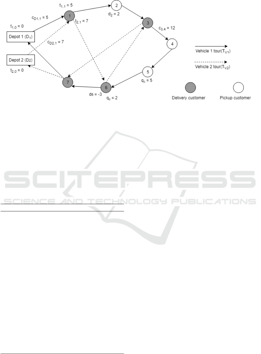
Figure 1: Synchronized vehicle tours.
3 SIMULATED ANNEALING
ALGORITHM
In order to tackle the problem described above, we
propose a simulated annealing-based approach (Kirk-
patrick et al., 1983) (see Algorithm 1).
Simulated annealing is a well-known metaheuris-
tic which has been widely studied and gave satisfy-
ing results for several types of optimization problems,
including VRP’s (Chiang and Russell, 1996) (Czech
and Czarnas, 2002) (Van Breedam, 1995).
Algorithm 1: Simulated annealing framework.
1: iterationsWithoutImprovement ← 0 ;
2: T ← T
0
;
3: S ← initialSolution() ;
4: bestSolution ← S ;
5: N ←
/
0 ;
6: while (iterationsWithoutImprovement <
maxIterations) do
7: iterationsWithoutImprovement + + ;
8: N ← Neighborhood(S) ;
9: S0 ← BestNeighbour(N) ;
10: ∆ ← f (S0) − f (S) ;
11: p ← Random(0,1) ;
12: if (p ≤ e
−∆/T
) then
13: S ← S
0
;
14: if ( f (S) ≤ f (bestSolution)) then
15: bestSolution ← S ;
16: iterationsWithoutImprovement ← 0 ;
17: end if
18: end if
19: T ← αT ;
20: end while
The main idea of simulated annealing is to try to
move, at each iteration, from a current solution S, to
a neighbour one S0 according to a certain probability
e
−∆/T
. This probability is updated at each iteration
and depends on two parameters:
• ∆ = f (S0)− f (S). If S0 improves S (if ∆ ≤ 0), then,
the probability to move to S0 is equal to 1. Other-
wise, the smaller ∆, the higher the probability to
move to S0;
• The temperature T . This parameter starts with
an initial value T
0
and decreases progressively at
each iteration. The greater T , the higher the prob-
ability to move to S0. In other words, the algo-
rithm is more likely to accept a candidate solution
S0 during the first iterations.
As it appears in Algo.1, the simulated annealing needs
an initial solution, and a heuristic to generate the
neighbourhood of the current solution at each itera-
tion.
3.1 Initial Solution
As an initial solution, we consider the solution ob-
tained by the “nearest neighbour algorithm”. Thus,
for the vehicle V
1
, we start from the depot D
1
at t = 0
and we move at each iteration to the nearest customer
from the current location of V
1
(in terms of travel
time) until all customers have been visited. The same
procedure is applied for V
2
: we start from D
2
and
move at each iteration to the nearest “delivery cus-
tomer”, until all delivery customers have been visited
by V
2
. Note that the departure time of V
2
from the
depot D
2
is set to t
1,i
− c
D
2
,i
, where i is the first cus-
tomer to be visited by V
2
, t
1,i
is the departure time of
V
1
from customer’s i location, and c
D
2
,i
the travel time
ICORES 2020 - 9th International Conference on Operations Research and Enterprise Systems
300

between D
2
and i. In other words, we choose the mo-
ment where V
2
leaves the depot to visit customer i in
such a way that both V
1
and V
2
arrive at the same time
at customer’s i location.
3.2 Neighbourhood Structure
We define a neighbour of a solution S as a solution
in which we swap the positions of two random cus-
tomers in one or both tours. Thus, to generate a neigh-
bour solution:
• We start by choosing 2 random customers i and j
among all the customers to be visited (including
“pickup” customers and “delivery” customers);
• If at least one of these customers is a “pickup”
customer (ie: he requires a visit of V
1
only), then
we swap the positions of i and j in V
1
’s tour;
• If the two chosen customers are “delivery” cus-
tomers (ie: they require a visit of both vehicles),
then we swap positions of i and j either in V
1
’s
tour, or in V
2
’s tour, or in both tours (we choose
randomly one of these three strategies).
So, as it is described in Figure 2, the neighbour so-
lution (on the right side) is obtained by swapping the
positions of customer 1 and customer 3. In the ini-
tial solution, customer 1 is the first customer to be
visited by both V
1
and V
2
, while customer 3 is at the
third position in V
1
’s tour, and at the second position
in V
2
’s tour. A neighbour solution is then generated
by moving customer 1 from positions [1,1] to [3,2]
and customer 3 from positions [3,2] to [1, 1].
4 COMPUTATIONAL RESULTS
The heuristic and the ILP model presented above were
implemented in Java and CPLEX 12.9. Both were
executed on AMD A10-7700K Radeon R7, 3.40 GHz
With 8 GB RAM.
To the best of our knowledge, there are no bench-
mark instances for simultaneous vehicle routing prob-
lems with pickup & delivery. Therefore, we tested
our algorithm on the Euclidian PDTSP instances gen-
erated by (Gendreau et al., 1999), which consider a
single depot for each instance. The benchmark con-
tains 180 instances where the number of customers
varies between 25 and 200. We adapted the instances
to fit our constraints by considering the depot and the
first customer of each instance as the depots of the two
vehicles considered in our problem.
However, to the best of our knowledge, there are
no papers dealing with the same problem as ours, so,
we have compared our results to the optimal solutions
found by our ILP model.
Concerning the simulated annealing parameters,
several values have been tested for the initial tempera-
ture T
0
and the parameter α. In the following, we con-
sider T
0
= 4800, α = 0.95, and maxIterations = 200.
Table 1 shows the average results obtained by our
simulated annealing for the 6 classes of instances (25,
50, 75, 100, 150, and 200 nodes).
The first column represents the class of instances
(the number of nodes), the second is the average to-
tal travel times obtained by our simulated annealing
on the 30 instances tested for each class. The third
column gives the average V
1
travel times, while the
fourth column represents the average V
2
travel times
(note that total travel times = V
1
travel times + V
2
travel times). The fifth column shows the average tar-
diness obtained by the algorithm. For each instance,
the sum of tardiness is the sum of the gaps between
the arrival time of V
1
and the arrival time of V
2
at each
customer’s location. In other words, given a solution,
tardiness =
∑
i∈N
d
t
2,i
−t
1,i
. Note that tardiness concerns
only “delivery” customers and its value is always pos-
itive because we have the constraint t
2,i
≥ t
1,i
. The last
column gives the CPU time in ms.
First, we note that the computational times are
very short, even for the largest instances. Further-
more, we see that pickup & delivery tours (vehicle V
1
)
are more costly than concrete delivery tours (V
2
) be-
cause they involve more customers. However, know-
ing that the number of customers visited by V
1
is about
the double of the number of customers visited by V
2
in the considered instances, the impact of V
2
’s tours
may appear relatively important (it represents more
than 40% of the total travel times for all classes of in-
stances). This can be explained by the fact that V
1
’s
tour are more flexible than V
2
’s ones, since V
2
is sub-
ject to a constraint that enforces it to do not visit a
customer before V
1
. Thus, good solutions may be re-
jected because they do not satisfy this constraint.
Table 2 shows a comparison between simulated
annealing results and the optimal solutions found by
our ILP model. Note that we could not obtain opti-
mal solutions in reasonable time for large instances
(≥ 75). Thus, in the following table, we do not
compare all the instances as in table 1, only 14 in-
stances have been compared, the first 10 instances of
25 nodes, and the first 4 instances of 50 nodes.
First, we observe that our simulated annealing ob-
tained very satisfying results. The solutions found are
globally close to optimal solutions, and the computa-
tional times are very much shorter (up to x 27000).
Furthermore, for large instances, optimal solutions
could not be obtained in reasonable time, contrary to
Simulated Annealing Approach for the Vehicle Routing Problem with Synchronized Visits
301

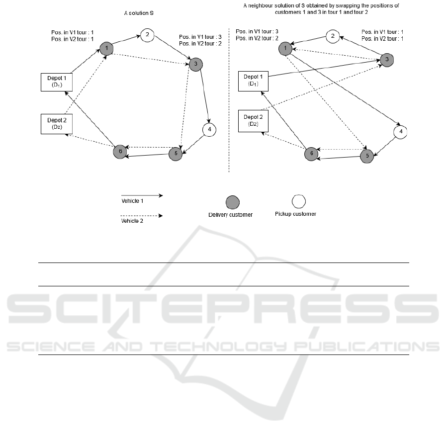
Figure 2: Neighbourhood generation.
Table 1: Simulated annealing results for the instances of (Gendreau et al., 1999).
Number
of nodes
Total
travel times
Pickup & delivery
tour (V1)
Concrete delivery
tour (V2)
Tardiness
CPU time
(ms)
25 908 530 (58%) 377(42%) 2461 95
50 1266 685 (54%) 580 (46%) 9276 457
75 1467 837(57%) 629 (43%) 21148 1046
100 1692 967 (57%) 724 (43%) 32761 2029
150 2047 1216 (57%) 830 (43%) 59562 6719
200 2451 1462 (57%) 988 (43%) 93546 18198
our heuristic which is effective for large instances (see
Table 1).
On the other hand, we note that the solutions
found by our heuristic present globally less tardiness
than the optimal ones. In other words, waiting times
between the visits of V
1
and V
2
at each customer’s lo-
cation are globally shorter with our simulated anneal-
ing solutions, which is interesting from the customer’s
point of view. Finally, we observe that the concrete
delivery tours (V
2
) obtained by the simulated anneal-
ing are much closer to optimal tours than the pickup
& delivery tours (V
1
). This is due to the fact that V
2
has a smaller set of customers to visit, which makes
the search space smaller for the heuristic. Moreover,
the fact that V
2
’s tours are more optimized than V
1
’s
tours can explain why the tardiness is globally shorter
with the solutions obtained by the simulated anneal-
ing. Indeed, if V
2
has a more optimized route than
V
1
, it would be more difficult to have a large gap be-
tween V
1
and V
2
, knowing that V
1
has more customers
to visit.
5 CONCLUSIONS
We presented a simulated annealing and an ILP model
to tackle the vehicle routing problem with synchro-
nized visits. The problem involves two vehicles:
the first has to visit n customers to pickup or de-
liver empty containers, while the second has to de-
liver ready-mixed concrete by pouring it into the pre-
viously delivered containers. The objective func-
tion considered is the minimization of the total travel
times.
We tested our algorithm and ILP model on the Eu-
clidian PDTSP instances proposed in (Gendreau et al.,
1999). We adapted the instances to fit our constraints
and collected the results, which were satisfying both
in terms of computational times and in terms of solu-
tion quality.
Future works will be devoted to the development
of multi-objective approaches including the mini-
mization of the total travel times and the minimization
of the tardiness.
ICORES 2020 - 9th International Conference on Operations Research and Enterprise Systems
302

Table 2: Simulated annealing solutions VS optimal solutions (ILP).
ILP solutions Simulated annealing solutions
Instance
CPU
time (ms)
Total
travel
time
Pickup &
delivery
tour (V1)
Concrete
delivery
tour (V2)
Tardiness
CPU
time (ms)
Total
travel
time
Pickup &
delivery
tour (V1)
Concrete
delivery
tour (V2)
Tardiness
25 0 13343 688 388 300 2037 218 816 510 306 966
25 1 15140 791 460 331 2152 109 991 641 350 2665
25 2 421 828 464 364 4838 109 990 524 466 4731
25 3 2375 789 464 325 3249 78 978 603 375 3113
25
4 12531 754 426 328 2035 62 801 467 334 1280
25 5 43703 806 453 353 3663 62 1018 600 418 2781
25 6 9656 771 440 331 1394 78 829 488 341 3960
25 7 569734 820 448 372 4298 109 1037 578 459 1111
25 8 19171 730 432 298 2722 78 820 468 352 760
25 9 104328 755 420 335 341 93 855 495 360 1685
50 0 526156 1035 581 454 9608 468 1268 742 526 9222
50 1 224953 1030 599 431 6300 312 1268 709 559 9964
50 2 13504468 968 553 415 11561 500 1154 658 496 7368
50 3 3533703 1071 595 476 12570 562 1231 651 580 8599
50 4 1179000 1007 574 433 10113 484 1206 722 484 10005
Other types of metaheuristics will be also studied,
such as genetic algorithms, and more constraints will
be involved including vehicle capacity constraints and
time windows.
REFERENCES
Afifi, S., Dang, D.-C., and Moukrim, A. (2016). Heuris-
tic solutions for the vehicle routing problem with time
windows and synchronized visits. Optimization Let-
ters, 10(3):511–525.
Bredstr
¨
om, D. and R
¨
onnqvist, M. (2008). Combined vehi-
cle routing and scheduling with temporal precedence
and synchronization constraints. European journal of
operational research, 191(1):19–31.
Chiang, W.-C. and Russell, R. A. (1996). Simulated an-
nealing metaheuristics for the vehicle routing problem
with time windows. Annals of Operations Research,
63(1):3–27.
Czech, Z. J. and Czarnas, P. (2002). Parallel simulated
annealing for the vehicle routing problem with time
windows. In Proceedings 10th Euromicro workshop
on parallel, distributed and network-based process-
ing, pages 376–383. IEEE.
Dohn, A., Rasmussen, M. S., and Larsen, J. (2011). The
vehicle routing problem with time windows and tem-
poral dependencies. Networks, 58(4):273–289.
Gendreau, M., Laporte, G., and Vigo, D. (1999). Heuris-
tics for the traveling salesman problem with pickup
and delivery. Computers & Operations Research,
26(7):699–714.
Hojabri, H., Gendreau, M., Potvin, J.-Y., and Rousseau, L.-
M. (2018). Large neighborhood search with constraint
programming for a vehicle routing problem with syn-
chronization constraints. Computers & Operations
Research, 92:87–97.
Kirkpatrick, S., Gelatt, C. D., and Vecchi, M. P. (1983).
Optimization by simulated annealing. science,
220(4598):671–680.
Lenstra, J. K. and Kan, A. R. (1981). Complexity of ve-
hicle routing and scheduling problems. Networks,
11(2):221–227.
Liu, R., Tao, Y., and Xie, X. (2019). An adaptive large
neighborhood search heuristic for the vehicle routing
problem with time windows and synchronized visits.
Computers & Operations Research, 101:250–262.
Sarasola, B. and Doerner, K. F. (2019). Adaptive large
neighborhood search for the vehicle routing problem
with synchronization constraints at the delivery loca-
tion. Networks.
Van Breedam, A. (1995). Improvement heuristics for the
vehicle routing problem based on simulated anneal-
ing. European Journal of Operational Research,
86(3):480–490.
Simulated Annealing Approach for the Vehicle Routing Problem with Synchronized Visits
303