
Real-time Surveillance based Crime Detection for Edge Devices
Sai Vishwanath Venkatesh
1 a
, Adithya Prem Anand
2 b
, Gokul Sahar S.
2 c
,
Akshay Ramakrishnan
2 d
and Vineeth Vijayaraghavan
3
1
SRM, Institute of Science and Technology, Chennai, India
2
SSN, College of Engineering, Chennai, Tamil Nadu, India
3
Solarillion Foundation, Chennai, Tamil Nadu, India
{vsaivishwanath, adithya.prem98, gokulsahar, akshayramakrishnan10}@gmail.com, vineethv@ieee.org
Keywords:
Real-time, Surveillance, Edge Devices, Resource-constrained, Crime Detection.
Abstract:
There is a growing use of surveillance cameras to maintain a log of events that would help in the identifi-
cation of criminal activities. However, it is necessary to continuously monitor the acquired footage which
contributes to increased labor costs but more importantly, violation of privacy. Therefore, we need decen-
tralized surveillance systems that function autonomously in real-time to reduce crime rates even further. In
our work, we discuss an efficient method of crime detection using Deep Learning, that can be used for on-
device crime monitoring. By making the inferences on-device, we can reduce the latency, the cost overhead
for the collection of data into a centralized unit and counteract the lack of privacy. Using the concept of Early-
Stopping–Multiple Instance Learning to provide low inference time, we build specialized models for crime
detection using two real-world datasets in the domain. We implement the concept of Sub-Nyquist sampling on
a video and introduce a metric η
comp
for evaluating the reduction of computation due to undersampling. On
average, our models tested on Raspberry Pi 3 Model B provide a 30% increase of accuracy over benchmarks,
computational savings as 80.23% and around 13 times lesser inference times. This allows for the development
of efficient and accurate real-time implementation on edge devices for on-device crime detection.
1 INTRODUCTION
In the past decade, the number of violent crime rates
has reduced across the globe (UNODC, 2017). Re-
ports (Alexandrie, 2017) (Piza et al., 2019) suggest
that this can majorly be attributed to the explosive
rise in the number of surveillance systems being em-
ployed. However, with this burgeoning rise comes
problems that need solving. Apart from the cost of in-
stalling surveillance systems, monitoring surveillance
feed is a recurring investment that makes surveillance
installation questionable of value to its stakeholders.
Monitoring surveillance also poses major privacy is-
sues. Policymakers and governments hesitate to up-
scale existing surveillance systems due to the increase
in labor cost and inevitable social unrest that could
be caused by the decrease in public privacy. How-
ever, according to the report (Nancy G. La Vigne and
a
https://orcid.org/0000-0001-6568-6259
b
https://orcid.org/0000-0002-3420-8809
c
https://orcid.org/0000-0002-1318-2216
d
https://orcid.org/0000-0001-6861-5675
Dwyer, 2015), police officials state more crimes are
deterred by active surveillance monitoring and inter-
vening. This begs for the need for better surveillance
monitoring techniques that can preserve privacy as
well as offer fast crime detection for immediate inter-
vention.The authors of this paper propose a real-time
edge implementation for surveillance based crime de-
tection to address the aforementioned needs.
This paper is organized as follows: Section 2
discusses the related research work carried out in
crime detection and edge research. The data used
for experimentation is described in Section 3 and
the methods employed for efficient feature extrac-
tion is compared in Section 4. Section 5 briefly
explains Early Stopping-Multiple Instance Learning
techniques implemented. Model implementation and
selection of model parameters are elucidated in Sec-
tion 6 followed by the results obtained and evaluation
of said models against benchmarks from contempo-
rary works in Section 7.
2 BACKGROUND
Video Action Recognition is currently one of the most
prominent fields of research in Computer Vision.
Brendel et al. presented an exemplar-based approach
to detect activities in realistic videos by considering
them as a time series of human postures (Brendel
and Todorovic, 2010). Simonyan et al. used a two-
stream convolutional network for capturing spatial
and temporal representations of videos and employed
multi GPU training of these representations for activ-
ity recognition (Simonyan and Zisserman, 2014). Ac-
tivity recognition has also been extended to analyze
the anomalies in surveillance videos. Sultani et al.
used 3D Convolution (C3D) and Tube-CNN (TCNN)
models to classify crimes in surveillance videos by
detecting anomalies (Sultani et al., 2018). Tay et
al. proposes an image-based Convolutional Neural
Network for the identification of abnormal activities
present in the video (Tay et al., 2019). Zhu et al.
proposes a motion aware feature using autoencoders
to detect anomalies in videos more effectively (Zhu
and Newsam, 2019). However, existing surveillance
video activity detection models require a lot of over-
head given that the recorded data has to be sent to a
centralized server for processing (Cui et al., 2019).
This can be eliminated by using compressed edge-
based models for prediction thereby enabling decen-
tralized implementations.
In the recent past, we have seen a significant in-
crease in edge oriented research with the implementa-
tion of powerful Machine Learning and Deep Learn-
ing models on these devices. Machine Learning al-
gorithms like k-Nearest Neighbours (kNN) and tree-
based algorithms have paved way for the develop-
ment of novel algorithms like ProtoNN (Gupta et al.,
2017) and Bonsai (Kumar et al., 2017) which ad-
dress the problem of real-time prediction on resource-
constrained devices by significantly reducing the
model size and inference time. Meng et al. proposed
an alternative for deploying computationally expen-
sive models on resource-constrained devices by intro-
ducing a Two-Bit Network (TBN) which helps in the
compression of large models like CNN (Meng et al.,
2017). Dennis et al. proposed a new method of Multi-
ple Instance Learning with Early Stopping to work on
sequential data which can be used for edge implemen-
tation of deep models like RNN and LSTM (Dennis
et al., 2018).
In our work, we have proposed a method that
enables real-time crime detection by encompassing
video action recognition strategies with edge device
compatibility without any compromise on accuracy.
3 DATASET
Since we aim to achieve effective on-device crime
detection for real-world surveillance, parameters like
the number of videos for analysis, presence of re-
alistic anomalies and proper annotations of videos
are taken into consideration to decide the data to be
used for our experiments. On this basis, we select 2
datasets — UCF-Crime and Peliculas — for our work.
Table 1: Dataset Description.
Parameter UCF-Crime Peliculas
# of videos 1900 (749 used) 203
# of classes 13 (8 used) 2
Frames per
second(fps)
30 30
Average
Frames
7247 (4 mins) 50
Frame aspect
Ratio
240×320 px 240×320 px
Annotated Yes Yes
3.1 UCF-Crime
The videos in this dataset have been sourced by the
University of Central Florida (UCF) (Sultani et al.,
2018) using search queries of different languages
from broadcasting platforms such as YouTube and
LiveLeak. Furthermore, videos in the dataset have
been resized to a standard 240×320 pixels and are
sampled at a frame rate of 30 frames per second (fps).
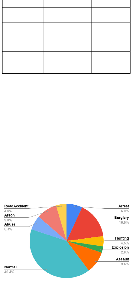
The crimes labeled within these videos include
eight classes namely Assault, Arson, Fighting, Bur-
glary, Explosion, Arrest, Abuse and Road Accidents.
Additionally, the collection contains Normal videos,
i.e., videos that do not contain any crime footage. The
class-wise distribution of the percentage of videos in
each class of UCF-Crime is illustrated in Figure 1.
Figure 1: Class-wise percentage of frames in UCF-Crime.
3.2 Peliculas
Peliculas (Gracia et al., 2015) is a binary class dataset
consolidated by Gracia et al. contains real-world
fighting videos and non-fight videos taken from UCF
101 (Soomro et al., 2012), the Hockey Fighting
dataset (Nievas et al., 2011) as well as fight scenes
from the Movies Dataset (Nievas et al., 2011). Fur-
thermore, these videos have been resized to a standard
240×320 pixels and each video is sampled at a frame
rate of 50 fps.
Table 1 describes the parameters of the datasets
considered.
4 ANALYSIS OF FEATURE
EXTRACTION TECHNIQUES
Videos can be interpreted as a sequence of frames
that contain spatial and temporal elements (Laptev
et al., 2008). For effective activity recognition, the
extracted features must capture both elements for a
set of frames. Since we wish to implement our work
in real-time, we aim to minimise the computational
cost of feature extraction methods used.
4.1 Histogram of Oriented Gradients
Histogram of Oriented Gradients (HOG) is an image
processing technique that captures the spatial orienta-
tion of pixels in an image. It is widely used in human
detection (Dalal and Triggs, 2005) and pose estima-
tion (Brendel and Todorovic, 2010) to recognize ac-
tions from a single high resolution image. Although it
captures spatial features, HOG is incapable of captur-
ing the essential temporal elements required for video
activity recognition.
4.2 Deep Spatio-temporal Extraction
In this method, each frame from the video is taken and
passed through a pre-trained deep learning model.
The values from the penultimate layer of the pre-
trained deep model yield useful spatial information as
illustrated in (He et al., 2016; Pratt, 1993). This archi-
tecture can be extended to gather temporal features.
Some of the work that use this technique include
C3D (Tran et al., 2015), VTN (Girdhar et al., 2019)
and I3D (Carreira and Zisserman, 2017). However,
since these models have extremely deep architec-
tures due to several models being pipelined, they
prove to be significantly slower than other methods as
seen in Table 2 and incapable of efficient edge
implementation.
4.3 Histogram of Optical Flow
Histogram of Optical Flow is an image processing
technique that captures both spatial and temporal fea-
tures of a video. We define such features as spatio-
temporal features. Optical Flow is the pattern of ap-
parent motion of the different entities in a video. Cal-
culating the histogram of optical flow across the video
frames yields values that can serve as features that
encompass the temporal variations in between two
frames. The process of calculating HOF is shown
in Figure 2 where the vector magnitudes and orienta-
tions are coded using the HSV model for visualization
purposes. Optical flow estimation algorithms can be
broadly classified into two main categories based on
the density of points considered namely Sparse Opti-
cal Flow and Dense Optical Flow.
4.3.1 Sparse Optical Flow
In this method, the optical flow is estimated on certain
selected points within the frame under consideration.
Lucas-Kanade proposes (Lucas et al., 1981) one such
sparse optical flow estimation method.
u
v
=
∑
i
f
2
x
i
∑
i
f
x
i
f
y
i
∑
i
f
x
i
f
y
i
∑
i
f
2
y
i
−1
−
∑
i
f
x
i
f
t
i
−
∑
i
f
y
i
f
t
i
(1)
Equation 1 gives the formula for the calculation of u
and v, i.e., optical flow coefficients for a particular
point (x,y,t). Here, x, y and t represent the coordinates
of a pixel in space-time.
Since sparse optical flow considers the optical flow
only for certain points, it results in a different number
of features for a different set of frames. This gives us
a reason to shift our attention towards dense optical
flow.
4.3.2 Dense Optical Flow
Dense Optical Flow is an optical flow estimation tech-
nique that considers the whole frame for the esti-
mation. Unlike sparse optical flow, dense optical
flow produces a fixed length of features provided the
frames fed into the algorithm have a constant aspect
ratio. We use the dense optical flow algorithm given
in (Farneb
¨
ack, 2003). One of the reasons for adopting
this method is its ability to take every nuance in the
frame for the extraction of features.
f
1
(x) = x
T
A
1
x + b
T
1
x + c
1
(2)
f
2
(x) = f
1
(x + d)
= x
T
A
2
x + b
T
2
x + c
2
(3)
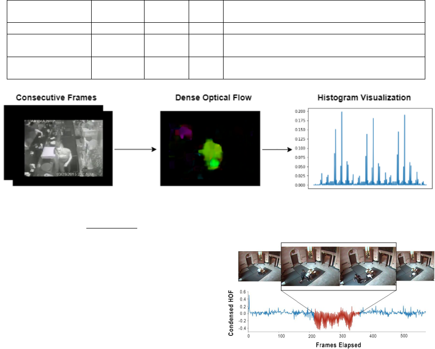
Table 2: Comparison of Feature Extraction Properties.
Method
Time
Taken(ms)
Features
Length
Cores
Used
Miscellaneous
HOF (Dense) 6.36 540 1 Spatio-temporal Features extracted
HOG 0.74 324 1
Only spatial information encoded
Fastest among the methods considered
Deep-Spatio
Temporal (Resnet)
42.36 512 4 Requires extra memory to store pretrained model
Figure 2: Histogram of Optical Flow.
d =
A
−1
1
(b
2
− b
1
)
2
(4)
where,
f represents a frame,
A
i
is a symmetric matrix,
b
i
is a vector,
c
i
is a scalar.
d is the global displacement from frame f
1
(Equation
2) to frame f
2
(Equation 3).
Here, f
1
and f
2
represent the subsequent frames
from the video considered for the estimation of op-
tical flow. In (Farneb
¨
ack, 2003), every frame con-
sidered for optical flow estimation is resolved into a
quadratic equation as shown in Equation 2.
Based on the comparative study (Table 2), we can
conclude qualitatively that Histogram of Optical Flow
is best suited for video activity recognition since it
provides temporal information. Due to conclusions
drawn in Section 4.3.1 we consider a dense imple-
mentation for our experiments over sparse.
4.4 Time Series Analysis - HOF
Principal Component Analysis (Pearson, 1901) is
used to condense HOF features into one dimension
for representational ease. Representing HOF in this
format helps us to observe its similarities to one-
dimensional time series. We can observe from Figure
3 that HOF displays characteristics representative of
time series data.
Time series data refers to a set of observations ob-
tained sequentially over time such as sensor readings
(Anguita et al., 2012) or stock market prices (Agarwal
and Sabitha, 2016). With reference to our work, time
corresponds to consecutive frames in a video.
Figure 3: Time series representation of HOF across a crime.
Furthermore, we believe our representational
HOF poses distinctive similarities to waveforms illus-
trated by other time series class recognition datasets
such as sensor-based Human Activity Recognition
(HAR) (Anguita et al., 2013) and Wake Word Dataset
(Warden, 2018). These waveforms are visibly distin-
guishable between different classes over a period of
time as observed in Figure 3. Also another similar-
ity between these datasets is that these are sparsely
annotated with activities. For example, HAR labels
human activities amongst noise, while UCF Crime la-
bels crimes as actions against normal videos.
This time-series data can be processed by Recur-
rent Neural Networks and LSTMs, which have proven
to discern activities on these type of data. However,
conventional RNNs and LSTMs require us to ana-
lyze the entire timestep before we make a predic-
tion. So we adopt Dennis et al.s’ (Dennis et al., 2018)
operationalised implementation of Multiple Instance
Learning (MIL) with Early Stopping (EMI).
5 EARLY STOPPING - MULTIPLE
INSTANCE LEARNING
5.1 Multiple Instance Leaning
Multiple instance learning (MIL) is a semi-supervised
method of learning used in pattern recognition espe-
cially to train sparsely annotated sequential data for
classification. It involves grouping sequential train-
ing records into batches called as bags (χ
i
). Each
bag is broken down into multiple overlapping sets
of instances of a constant width ω as seen in Fig 4.
These set of instances are called sub-instances (Z
i,τ
).
An entire bag is tagged with a singular label to rep-
resent its class. A set of sub-instances within the
bag that uniquely identifies the class is defined as
the class signature and is illustrated in Figure 4. We
choose a value k to represent the number of overlap-
ping set of sub-instances that encompasses the class
signature. These instances are considered positive in-
stances meanwhile the other instances in the bag are
considered as noise. Through MIL, we obtain a re-
duced training set by pruning bags to contain only
positively labeled instances (χ
P
i
). This increases the
chance of a higher prediction probability during the
testing phase.
Figure 4: Multiple Instance Learning.
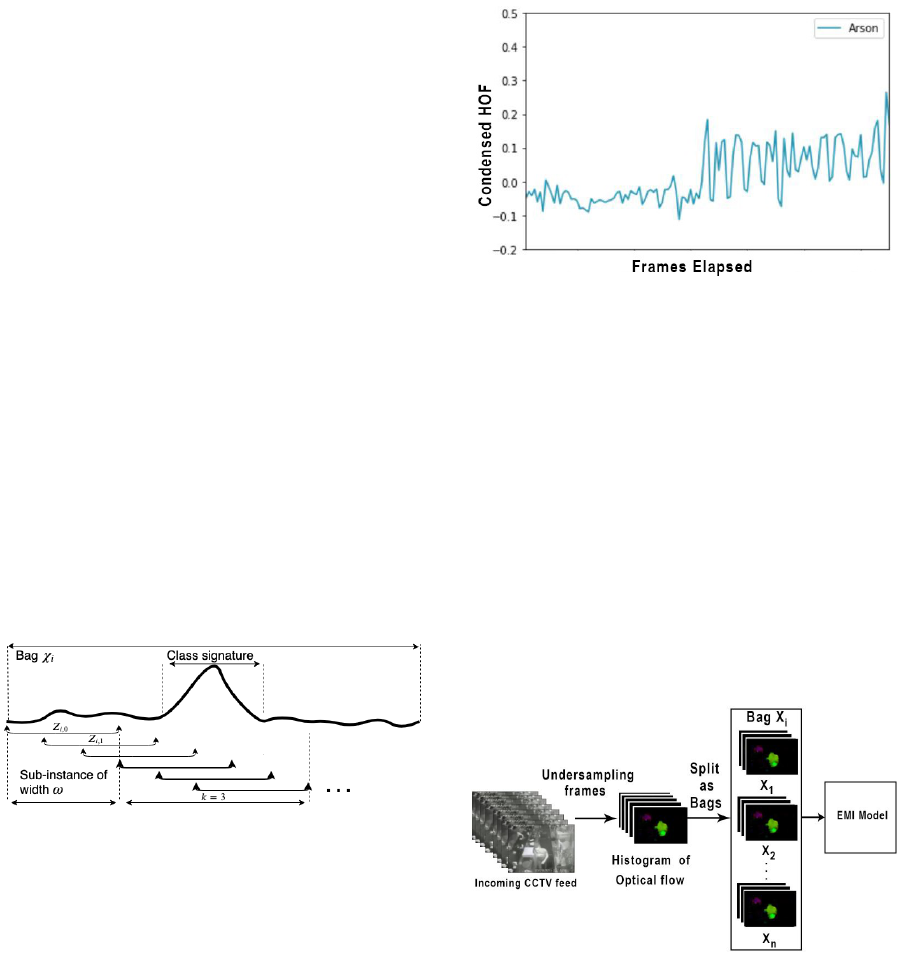
For example, the act of pouring gasoline could
represent the class signature for a bag that is labeled
Arson. Hence we can categorize an entire bag as Ar-
son by recognizing the class signature - pouring gaso-
line. Figure 5 illustrates two visible class signatures
for the label Arson namely ”pouring gasoline” and
”fire”.
5.1.1 Early Stopping
The early prediction implemented in our work serves
to improve a model’s inference time by stopping the
testing process early for a bag if the predicted proba-
bility for a class is greater than a desirable threshold
probability (confidence level). This is performed iter-
atively for each instance in a test bag until the afore-
mentioned condition is met or until the end of the bag.
Figure 5: Class signature.
Since this algorithm works after MIL provides an al-
ready pruned set of bags, the confidence level is sur-
passed within exponentially less number of iterations
and thus results in lesser inference time than normal.
6 METHODOLOGY
In this section, we elucidate the implementation of
Early Stopping and Multiple Instance Learning to de-
tect crime in surveillance videos. We penalize longer
inference times and larger model sizes since we aim
to optimize crime detection on edge devices. There-
fore, we make all our considerations regarding param-
eters and sampling rates to maximize testing accuracy
based on the aforementioned conditions.
Figure 6: Model Architecture.
6.1 Data Preprocessing
The sequence of images processed for the UCF-Crime
and Peliculas dataset is of the resolution 240×320
pixels and resized to half its size (120×160 pixels) in
order to reduce the computational overhead to obtain
a feature array for an image. By retaining the same
aspect ratio for frame resizing we reduce the HOF ex-
traction time for the video by half without incurring a
heavy loss in feature integrity. MIL requires a con-
stant set of variables that are a function of time (time
series). Therefore, we use the Dense representations
of HOF over variable-length Sparse representations of
HOF such as Spatio Temporal Interest Points (STIPs)
that provide an inconsistent number of STIPs across
frames (Laptev et al., 2008).
6.2 Undersampling
Frames per second (fps) is the sampling frequency of
the video under consideration. All UCF-Crime and
Peliculas videos are rendered in 30 frames per sec-
ond which we believe to be excessive for resource-
constrained HOF implementation. For our case, we
consider the possibility of interpreting the video by
sampling it at a Sub-Nyquist rate, i.e., frequency less
than the proposed value, with a reduction factor r as
given in Equation 5. Consequently, the number of
frames processed by MIL in a bag reduce by a fac-
tor of r as well. Reduction of fps with increase in r is
illustrated in Table 3. The implications of fps reduc-
tion are discussed in detail in Section 7.2.1 .
f =
f
s
r
, r ∈ N
(5)
where
f
s
is the ideal fps (or) sampling frequency
Table 3: Variation of Frames per Second with Reduction
Factor.
Reduction
Factor(r)
1 2 3 4 5 6
Frames per
second(fps)
30 15 10 7 6 5
6.3 EMI Parameters
6.3.1 Bag Size and Subinstance Width
After preprocessing the frames as 540 features of
dense HOF. We have to prepare the data to implement
Early Stopping - MIL by grouping extracted frames
into fixed-length bags. The length of each bag is re-
ferred to as bag size. As discussed in Section 5.1,
each bag encompasses a class signature. Therefore
we select the bag size to be intuitively longer than the
length of most class signatures within the dataset. To
enable training we need to remove several frames at
the end of a video since it is less than the bag size. The
corresponding loss in training data due to removal is
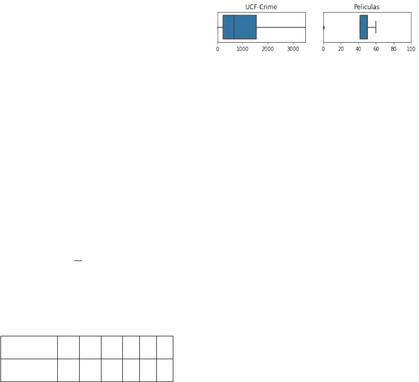
calculated using Equation 6. Figure 7 gives an insight
on the duration for which an event occurs in a video.
Knowing the distribution of the number of frames per
video (Figure 7) assists us in determining the bag size
Figure 7: Distribution of Annotated Video Durations.
for maximizing the accuracy as well as reduce the
incurred data loss. On this basis, we choose a bag
size of 128 frames for UCF-Crime and 24 frames for
Peliculas.
L = F − n × T, n ∈ N (6)
where,
L is the incurred data loss,
F is the total number of frames in the video,
T is the bag size,
n is the total number of bags
A smaller portion of the bag called the subin-
stance [Section 5.1] is fixed as 64 for UCF- Crime
dataset and 12 for Peliculas dataset.
6.4 EMI Implementation
Once the required parameters are set, the data is now
ready to be fed to the model. The three models that
are used with the concept of Multiple Instance Learn-
ing and Early Stopping are – EMI-LSTM, EMI-GRU,
and EMI-FastGRNN (Dennis et al., 2018) (Kusupati
et al., 2018). LSTMs and GRUs are the popular RNN
architectures that are used for the classification of se-
quential points. FastRNN and FastGRNN (Kusupati
et al., 2018) were developed to satiate the inefficien-
cies of RNN by employing residual connections. Due
to the weight matrix of FastGRNN being low rank,
sparse and quantized, it occupies less space compared
to other models.
7 RESULTS AND OBSERVATIONS
We deploy HOF feature extraction and EMI models
on the Raspberry Pi 3 Model B to prove the veracity
of their performance in realistic scenarios. The com-
putational environment of our work is illustrated in
Table 8.
7.1 Evaluation Metrics
Accuracy (F1 Score), Operation Time (seconds) and
Model Size (Mb) are considered as ideal metrics
of evaluation to collectively describe the efficiency

Table 4: UCF-Crime Optimization [L:EMI-LSTM; G:EMI-GRU; F:EMI-FastGRNN].
Reduction
Factor(r)
Frames per
second(fps)
Bag
Size
Sub-instance
width
Accuracy(%)
Inference
Time(s)
η
comp
L G F L G F L G F
1 30 128 64 95 95 86 7.16 7.6 6.87 - - -
2 15 64 32 94 93 83 3.82 3.97 3.44 46.6 47.7 49.9
4 7 32 16 88 85 75 1.97 1.99 1.98 72.5 73.8 71.2
6 5 21 10 91 89 78 1.36 1.37 1.30 77.8 81.9 81
Table 5: Peliculas Optimization [L:EMI-LSTM; G:EMI-GRU; F:EMI-FastGRNN].
Reduction
Factor(r)
Frames per
second(fps)
Bag
Size
Sub-instance
width
Accuracy(%)
Inference Time(s)
η
comp
L G F L G F L G F
1 30 24 12 99 99 97 1.654 1.678 1.652 - - -
2 15 12 6 97 95 90 0.852 0.825 0.824 48.3 51 50
4 7 6 3 99 99 93 0.412 0.413 0.412 75 75.4 75
of models running on resource-constrained devices.
Time refers to the sum of feature extraction time and
the EMI model inference time. Furthermore, we in-
troduce η
comp
to illustrate the computational savings
offered by our methods of optimization.
7.1.1 Computational Savings (η
comp
)
Computational Savings is indicative of the fraction of
optimized inference time to default.
η
comp
=
I
A
− I
R
I
A
× 100 (7)
where,
I
A
is the inference time using ideal fps for 1 bag,
I
R
is the inference time using reduced fps for 1 bag
7.2 Our Model
7.2.1 Undersampling Optimisation
We can observe how the reduction of frames (Section
6.2) affects the metrics of evaluation. When we con-
sider reduction factor (r ) ranging from 2-6 for UCF-
Crime, we observe an admissible decrease in accuracy
as illustrated in Table 4 (Average 6% across models)
with an average 32% increase in computational sav-
ings between r=2 and r=6. The average inference
time for maximum reduction r=6 across models for
UCF-Crime is 1.36 seconds. When reduction fac-
tor based optimisation was performed for the Pelic-
ulas Dataset (Section 3.2) the computational savings
shown in Table 5 increased by 25% between r=2 and
r=4. The lesser savings could be attributed to the
dataset’s low bag size.
7.3 Benchmarks
When we compare our model besides benchmarks es-
tablished for the datasets considered, we can evaluate
our model’s relative performance. Benchmark imple-
mentations include C3D (Tran et al., 2015) for UCF-
Crime and Fast Fight Detector (Gracia et al., 2015)
for the Peliculas dataset.
7.3.1 UCF-Crime
The EMI-LSTM, EMI-GRU, and EMI-FastGRNN
are implemented on UCF-Crime. Table 4 shows the
variation of model metrics with the reducing sampling
rate as given in Equation 5. Table 6 shows the met-
rics obtained for the dataset when the sampling rate
is reduced by a factor of 6. The FastGRNN model
occupies very little space being about 20 times lesser
than the benchmark model and is the fastest among
the models. LSTM offers the best accuracy.
Table 6: UCF-Crime Results.
Model
Accuracy
(%)
Inference
Time(s)
Size
(MB)
Benchmark 23.9 30 7.5
EMI-LSTM 91.3 1.36 1.3
EMI-GRU 89.1 1.31 1.0
EMI-FastGRNN 78.4 1.30 0.334
7.3.2 Peliculas
The EMI-LSTM, EMI-GRU, and EMI-FastGRNN
models are implemented for the Peliculas dataset, and
their performance is shown in Table 5. Table 7 shows
the metrics obtained for the dataset when the sam-
pling rate was reduced by a factor of 4. The EMI-

Table 7: Peliculas Results.
Model
Accuracy
(%)
Inference
Time(ms)
Benchmark 97.7 552
EMI-LSTM 99.2 412
EMI-GRU 99.0 413
EMI-FastGRNN 93.1 413
Table 8: Test Conditions.
Model Benchmark Ours
Processor Intel Xeon ARM v8
Number of cores 12 4
Processor Speed(GHz) 2.9 1.4
LSTM and EMI-GRU are very similar in their per-
formances but LSTM indicates an improved accuracy
score.
The test conditions of the benchmark and our
model are compared in Table 8. We implement our
solution with significantly fewer resources than the
benchmark.
8 CONCLUSION
Multiple Instance Learning and Early Stopping con-
cepts (EMI) were applied on two real-world crime
detection datasets and the feature extraction for the
same was optimized to have a faster extraction time
by sampling videos at a Sub-Nyquist rate. The
proposed models surpassed existing benchmarks and
have proven capable of being deployable on resource-
constrained technologies connected to surveillance
cameras. We achieved a maximum accuracy of
91.3%, inference time of 1.3s and a minimum model
size of 0.334MB in the UCF-Crime dataset. As far
as the Peliculas dataset is concerned, we achieved an
accuracy of 99.2% and an inference time of 412 ms.
ACKNOWLEDGEMENTS
The authors would like to acknowledge Solarillion
Foundation for its support and resources provided for
the research work carried out.
REFERENCES
Agarwal, U. and Sabitha, A. S. (2016). Time series forecast-
ing of stock market index. In 2016 1st India Interna-
tional Conference on Information Processing (IICIP).
Alexandrie, G. (2017). Surveillance cameras and crime:
a review of randomized and natural experiments.
Journal of Scandinavian Studies in Criminology and
Crime Prevention, 18(2):210–222.
Anguita, D., Ghio, A., Oneto, L., Parra, X., and Reyes-
Ortiz, J. L. (2012). Human activity recognition
on smartphones using a multiclass hardware-friendly
support vector machine. In International workshop on
ambient assisted living, pages 216–223. Springer.
Anguita, D., Ghio, A., Oneto, L., Parra, X., and Reyes-
Ortiz, J. L. (2013). A public domain dataset for human
activity recognition using smartphones. In Esann.
Brendel, W. and Todorovic, S. (2010). Activities as time
series of human postures. In European conference on
computer vision, pages 721–734. Springer.
Carreira, J. and Zisserman, A. (2017). Quo vadis, action
recognition? a new model and the kinetics dataset.
In proceedings of the IEEE Conference on Computer
Vision and Pattern Recognition, pages 6299–6308.
Cui, Y., Li, Q., Nutanong, S., and Xue, C. J. (2019). Online
rare category detection for edge computing. In 2019
Design, Automation & Test in Europe Conference &
Exhibition (DATE), pages 1269–1272. IEEE.
Dalal, N. and Triggs, B. (2005). Histograms of oriented
gradients for human detection.
Dennis, D., Pabbaraju, C., Simhadri, H. V., and Jain, P.
(2018). Multiple instance learning for efficient se-
quential data classification on resource-constrained
devices. In Advances in Neural Information Process-
ing Systems, pages 10953–10964.
Farneb
¨
ack, G. (2003). Two-frame motion estimation based
on polynomial expansion. In Scandinavian conference
on Image analysis, pages 363–370. Springer.
Girdhar, R., Carreira, J., Doersch, C., and Zisserman, A.
(2019). Video action transformer network. In Pro-
ceedings of the IEEE Conference on Computer Vision
and Pattern Recognition, pages 244–253.
Gracia, I. S., Suarez, O. D., Garcia, G. B., and Kim,
T.-K. (2015). Fast fight detection. PloS one,
10(4):e0120448.
Gupta, C., Suggala, A. S., Goyal, A., Simhadri, H. V.,
Paranjape, B., Kumar, A., Goyal, S., Udupa, R.,
Varma, M., and Jain, P. (2017). Protonn: compressed
and accurate knn for resource-scarce devices. In Pro-
ceedings of the 34th International Conference on Ma-
chine Learning-Volume 70, pages 1331–1340. JMLR.
org.
He, K., Zhang, X., Ren, S., and Sun, J. (2016). Deep resid-
ual learning for image recognition. In The IEEE Con-
ference on Computer Vision and Pattern Recognition
(CVPR).
Kumar, A., Goyal, S., and Varma, M. (2017). Resource-
efficient machine learning in 2 kb ram for the internet
of things. In Proceedings of the 34th International
Conference on Machine Learning-Volume 70, pages
1935–1944. JMLR. org.
Kusupati, A., Singh, M., Bhatia, K., Kumar, A., Jain, P.,
and Varma, M. (2018). Fastgrnn: A fast, accurate, sta-
ble and tiny kilobyte sized gated recurrent neural net-
work. In Advances in Neural Information Processing
Systems, pages 9017–9028.
Laptev, I., Marszałek, M., Schmid, C., and Rozenfeld,
B. (2008). Learning realistic human actions from
movies.
Lucas, B. D., Kanade, T., et al. (1981). An iterative image
registration technique with an application to stereo vi-
sion.
Meng, W., Gu, Z., Zhang, M., and Wu, Z. (2017). Two-bit
networks for deep learning on resource-constrained
embedded devices. arXiv preprint arXiv:1701.00485.
Nancy G. La Vigne, Samantha S. Lowry, J. A. M. and
Dwyer, A. M. (2015). Evaluating the use of pub-
lic surveillance cameras for crime control and preven-
tion—a summary.
Nievas, E. B., Suarez, O. D., Garc
´
ıa, G. B., and Sukthankar,
R. (2011). Violence detection in video using com-
puter vision techniques. In International conference
on Computer analysis of images and patterns, pages
332–339. Springer.
Pearson, K. (1901). Liii. on lines and planes of closest fit to
systems of points in space. The London, Edinburgh,
and Dublin Philosophical Magazine and Journal of
Science, 2(11):559–572.
Piza, E. L., Welsh, B. C., Farrington, D. P., and Thomas,
A. L. (2019). Cctv surveillance for crime prevention.
Criminology & Public Policy, 18(1):135–159.
Pratt, L. Y. (1993). Discriminability-based transfer between
neural networks. In Advances in neural information
processing systems, pages 204–211.
Simonyan, K. and Zisserman, A. (2014). Two-stream con-
volutional networks for action recognition in videos.
In Advances in neural information processing sys-
tems, pages 568–576.
Soomro, K., Zamir, A. R., and Shah, M. (2012). Ucf101:
A dataset of 101 human actions classes from videos in
the wild. arXiv preprint arXiv:1212.0402.
Sultani, W., Chen, C., and Shah, M. (2018). Real-world
anomaly detection in surveillance videos. In Proceed-
ings of the IEEE Conference on Computer Vision and
Pattern Recognition, pages 6479–6488.
Tay, N. C., Connie, T., Ong, T. S., Goh, K. O. M., and Teh,
P. S. (2019). A robust abnormal behavior detection
method using convolutional neural network. In Al-
fred, R., Lim, Y., Ibrahim, A. A. A., and Anthony,
P., editors, Computational Science and Technology,
pages 37–47, Singapore. Springer Singapore.
Tran, D., Bourdev, L., Fergus, R., Torresani, L., and Paluri,
M. (2015). Learning spatiotemporal features with 3d
convolutional networks. In Proceedings of the IEEE
international conference on computer vision, pages
4489–4497.
UNODC (2017). World crime trends and emerging is-
sues and responses in the field of crime prevention
and criminal justice. In 26th Edition, Commission on
Crime Prevention and Criminal Justice.
Warden, P. (2018). Speech commands: A dataset
for limited-vocabulary speech recognition. CoRR,
abs/1804.03209.
Zhu, Y. and Newsam, S. (2019). Motion-aware feature for
improved video anomaly detection.
