
Creating Curvature Adapted
Subdivision Control Meshes from Scan Data
Simon Kloiber
a
and Ursula H. Augsd
¨
orfer
Institute of Computer Graphics and Knowledge Visualisation,
Graz University of Technology, Inffeldgasse 16c, Graz, Austria
Keywords:
Quad-dominant Remeshing, Surface Reconstruction.
Abstract:
Often, designers have real-life models which need to be converted to a mathematical representation for fur-
ther processing. For the designer to be able to manipulate the data sensibly and in a controlled manner the
number of data points have to be reduced. However, if the new reduced representation of the shape is sparse
everywhere, high frequency detail in the model will be lost. In this work we modify an existing quad meshing
algorithm to convert a dense triangle mesh capturing the shape of the real-life model to a quad-dominant mesh
of varying density. Our distribution of vertices allows to represent high frequency features in the surface,
without increasing the density of the mesh elsewhere unnecessarily. Our quad mesh approximates the scan
data up to a predefined error margin. This quad mesh is then transformed into a subdivision control mesh,
which corresponds to a limit subdivision surface which closely resembles the scan data.
1 INTRODUCTION
Often, designers create real-life models of their ideas.
The real-life model is then scanned to obtain a dig-
ital representation in form of a point cloud, which
can be converted to a triangle mesh. Because these
meshes closely capture the shape of the real-life mod-
els, we will refer to these dense triangular meshes as
reference meshes. To be able to further refine the de-
sign within a design pipeline, a mathematical repre-
sentation of the shape has to be found. Subdivision
surfaces are able to model complex shapes with a
single surface. They are defined by a coarse set of
control points and a subdivision algorithm. To con-
tinue the design with subdivision surfaces, the ref-
erence mesh has to be converted into a subdivision
control mesh. The extraction of an adaptive subdivi-
sion control mesh from dense triangle meshes is the
focus in this paper. There are many different sub-
division schemes resulting in limit surfaces with dif-
ferent mathematical properties. While the algorithm
presented is applicable to any subdivision scheme, we
will base all examples on the Catmull-Clark scheme
since it is the de facto standard subdivision scheme in
the CAD and entertainment industry. Catmull-Clark
subdivision operates on quadrilateral meshes.
a
https://orcid.org/0000-0003-1186-7630
The paper is structured as follows. In Section 2 we
discuss related work on the topic of quad mesh gener-
ation. In Section 3 we describe how we extend an ex-
isting algorithm for isotropic quad meshing to create
non-uniform isotropic quad meshes that are sensitive
to the curvature of the surface and adapt the size of
the quadrilaterals such that the error of the extracted
quad-dominant mesh to the reference mesh does not
exceed a given threshold. We also describe a simple
way to convert a given quadrilateral polyhedron to a
Catmull-Clark control mesh so that the limit surface
closely describes the shape captured in the reference
mesh. We present our results in Section 4. We close
with the conclusion in Section 5.
2 QUADRILATERAL MESHING
Because Catmull-Clark subdivision is based on a
quadrilateral mesh, we first need to compute a quad
mesh (also called quadrangulation or quad meshing)
from a given input mesh. Quad meshing is a topic of
interest in many applications, like texture mapping,
parameterisation and finite element analysis and there
are numerous different approaches and methods. A
comprehensive survey is e.g. provided by (Bommes
et al., 2013b).
Quad meshing methods either define parametrisa-
Kloiber, S. and Augsdörfer, U.
Creating Curvature Adapted Subdivision Control Meshes from Scan Data.
DOI: 10.5220/0008989601490159
In Proceedings of the 15th International Joint Conference on Computer Vision, Imaging and Computer Graphics Theory and Applications (VISIGRAPP 2020) - Volume 1: GRAPP, pages
149-159
ISBN: 978-989-758-402-2; ISSN: 2184-4321
Copyright
c
2022 by SCITEPRESS – Science and Technology Publications, Lda. All rights reserved
149

tions or curves, or employ triangle decimation to cre-
ate quads. Parametrisations can be created through
global optimisations (Ray et al., 2006; Hormann and
Greiner, 2000; K
¨
alberer et al., 2007; Bommes et al.,
2009; Bommes et al., 2013a; Liu et al., 2011; Myles
et al., 2010) or by defining a coarse layout of charts
which are then parametrised (Tong et al., 2006; Dong
et al., 2006; Zhang et al., 2010; Zhang et al., 2013).
Another approach is defining curves on the reference
mesh in a cross-based layout. Creating pure quad
meshes is difficult with straightforward curve based
approaches because additional structures are needed
(Campen et al., 2012). Quad-dominant approaches
integrating curves are more prevalent (Alliez et al.,
2003; Marinov and Kobbelt, 2004; Dong et al., 2005).
A third approach employs triangle mesh decimation
(Lai et al., 2010), where quadrilateral faces are cre-
ated by combining triangles, and makes use of the fact
that creating a triangulation is easier than creating a
quadrangulation.
Some of these approaches allow anisotropy and
adapt the mesh density according to curvature:
(Zhang et al., 2010) create their pure quad mesh
via parametrising the quasi-dual Morse-Smale Com-
plex of a standing wave function with manual size
control. (Alliez et al., 2003) create quad-dominant
meshes from genus-0, non-closed input meshes. They
use a smoothed curvature tensor field to guide curves
in anisotropic regions and point sampling in spher-
ical regions. The layout of the curves (i.e. den-
sity, anisotropy, geometric accuracy) can be influ-
enced manually. (Marinov and Kobbelt, 2004) cre-
ate a parametrization on an arbitrary input mesh on
which curvature lines are traced. The traced lines sat-
isfy a manually set sampling density. (Dong et al.,
2005) create a smooth harmonic scalar field over the
mesh. They compute a gradient vector field and use a
second vector field which is orthogonal to the gradient
field to trace integral lines. The spacing of these lines
is curvature sensitive and may be controlled manu-
ally. (Lai et al., 2010) remesh the given triangle mesh
such that the density of the newly created triangle
mesh adapts to curvature. They then perform a re-
laxation on the triangle mesh which aligns the edges
of the triangles such that non-aligned edges can be
dropped to form curvature aligned quads. (Kovacs
et al., 2011) introduce an anisotropic metric to fea-
ture aligned and harmonic parametrisations. This im-
proves the approximation quality of these isotropic
approaches. The quad-dominant remeshing algorithm
by (Jakob et al., 2015) creates isotropic uniform quad-
dominant meshes through quick, local optimisation of
a parametrisation from triangle or point cloud refer-
ence meshes.
The results of uniform quad meshing methods
cannot create sparse subdivision control meshes that
have a low approximation error. We present a non-
uniform quad meshing method, which adapts the den-
sity of control points to the degree of detail present in
the original surface. To ensure an accurate representa-
tion of surface features, we adjust the size of mesh el-
ements to reflect curvature variations, but also aim to
align the mesh with shape features. This is achieved
by modifying the algorithm presented in (Jakob et al.,
2015) to respect the curvature detail of the original
scan data.
3 ADAPTIVE QUAD MESHING
This section provides a comprehensive guide through
our changes to Instant Meshes (Jakob et al., 2015).
We created a work-chain that is able to transform ref-
erence meshes into subdivision control meshes with
densities based on the curvature information of the
referenced surface. The local approach of optimising
the parametrization used by Instant Meshes is ideal
for using curvature information to shape the grid size
locally around each vertex. By adapting the local grid
size to the curvature of the shape we create a mesh
with large similar sized regular quadrilateral faces in
flat regions with low curvature, and small quadrilat-
eral faces in high curvature regions in order to cap-
ture high frequency details in the model. We con-
strain the orientation field estimation and feed the
edge lengths into the position field estimation. The
resulting mesh is post-processed to guarantee mani-
foldedness, to align quads with ridges, and to improve
the topology of flat areas. Finally, the extracted mesh
is transformed into a subdivision control mesh such
that its limit surface corresponds to the reference sur-
face given by the reference mesh.
The following steps are performed to extract
a quad-dominant subdivision control mesh with
curvature-based densities:
1. Build a multi-resolution hierarchy of the mesh.
For each hierarchy level, estimate the curvature,
compute the scales, and detect ridge vertices.
2. Optimise the orientation field.
3. Optimise the position field.
4. Extract the mesh.
5. Perform mesh clean-up.
6. Perform mesh smoothing.
7. Create the subdivision control mesh.
Changes in the density of Catmull-Clark subdivi-
sion control meshes are difficult to achieve because of
GRAPP 2020 - 15th International Conference on Computer Graphics Theory and Applications
150

their quad-based nature. Transitions from low to high
densities have to be done with care because they will
introduce additional extraordinary vertices (EVs). An
extraordinary vertex has a valency other than regular,
that is either more or less than four. Typically, the EVs
are avoided, since they are associated with curvature
problems in the limit surface. In this work, however,
we accept the appearance of EVs in order to capture
shape information encapsulated in high frequency re-
gions of the surface.
3.1 Curvature Estimation
There are two ways to estimate curvature on a piece-
wise linear mesh: Fitting parametric surfaces locally
around each vertex or estimating curvature in a dis-
crete sense based on the neighbourhood of a vertex
(Petitjean, 2002; Gatzke and Grimm, 2006). Paramet-
ric surface fitting generally produces better results at
the expense of computation time compared to other
methods. Most discrete methods are linear in time
because they compute sums over neighbours, but are
more susceptible to noise (Gatzke and Grimm, 2006).
We employ principal curvatures to fit a parametric
surface, because they are more precise and uniform
compared to other methods. The improved preci-
sion warranted the increased time complexity (a fac-
tor of three for an input mesh with 50000 vertices and
100000 faces).
The parametric surface fitting method of cubic or-
der developed in (Goldfeather and Interrante, 2004)
estimates principal curvature directions well and com-
putes satisfying results. To estimate the principal di-
rections and curvature, a cubic order B-spline patch
is fitted onto the neighbourhood of a vertex. For this,
neighbouring vertices are brought into a local coordi-
nate frame to create a system of equations where the
neighbours describe the shape of the parametric sur-
face. We found a 2-ring neighbourhood works well.
Every neighbouring point introduces three equations
with one equation for the position and two equations
for the normals. The least-squares solution of this sys-
tem of linear equations is the Weingarten curvature
matrix of the cubic surface. The Eigenvalues of this
matrix are the principal curvatures and its Eigenvec-
tors are the corresponding principal directions.
From the estimated curvature, we take the largest
absolute principal curvature as our guide for edge
lengths. This ensures that the highest frequency de-
tail is always respected.
3.2 Curvature Averaging
The curvature information might not be as smooth as
needed for good results. This may be due to noise in
the reference mesh or multiple different features com-
ing together in the mesh. To address these issues, we
tried different averaging methods to achieve a smooth
curvature distribution. We also tried different weigh-
ing schemes, either in order to increase the influence
of high curvature regions or based on similarity (be
it curvature or normal similarity). We found that uni-
form weights for all neighbours in a 2-ring neighbour-
hood produced the most consistent results.
3.3 Error Estimation and Edge Length
A scale parameter employed in the work of (Jakob
et al., 2015) defines a global desired edge length of
the extracted mesh. This scale influences the position
field calculation and the extraction itself. In the po-
sition field, the scale defines the positional invariance
points of the field while in the extraction it is used
to classify edges and to remove unnecessary edges.
To adjust scale based on curvature, the first step is
unravelling the global scale by giving each point its
own. The transformation of curvature to scale is a
one-dimensional map and is very similar to a simple
transfer function in volume rendering (Ljung et al.,
2016).
All information necessary to define a desired edge
length for a given vertex that fits the complexity of the
underlying surface is provided by the curvature esti-
mation. The relation of a tangent to the osculating
circle provides an error metric. We can use it to esti-
mate the error when moving along a curve in direction
of the tangent direction away from the vertex. As il-
lustrated in Figure 1, for a vertex v with curvature κ
along a tangential curve on the surface, the osculating
circle has radius
1
|κ|
. When we move away from the
point along this curve by x, we denote the estimated
distance to the curve as ε. Users can select the desired
error, which drives the edge length computation.
(Alliez et al., 2003) have used a similar estima-
tion that places the constructed edge such that its end-
points are on opposing sides of the circle (i.e. the
vertex is its centre). This way, the same error ε will
allow an edge length of 2x(ε). Their derivation creates
edges that are larger and become smaller too slowly.
Hence, the factor of two is not incorporated in our
edge length computation.
Because the derived edge lengths tend to infin-
ity as the curvature approaches zero, we cap edge
lengths to remain smaller than five times the global
edge length. In areas where the edge length is too
Creating Curvature Adapted Subdivision Control Meshes from Scan Data
151

r =
1
|κ|
r
2
= (r − ε)
2
+ x
2
x
2
= r
2
− (r − ε)
2
x
2
=
1
|κ|
2
− (
1
|κ|
− ε)
2
x
2
=
2
|κ|
ε − ε
2
x(ε) =
s
2
|κ|
ε − ε
2
0 ≤ ε ≤
1
|κ|
ε
1
κ
v
x
Figure 1: The derivation of the maximum edge length x(ε)
with an error of ε, for tangential edges going out of vertex v
with curvature κ.
small for the density of the reference mesh, the posi-
tion field can either not form clusters or forms clus-
ters that are too small to extract vertices. If not spec-
ified differently by a user, (Jakob et al., 2015) set the
global edge length such that the expected number of
extracted vertices is 1/16th of the number of refer-
ence vertices. This expectation has become less pre-
cise due to varying quad sizes but is still a good in-
dicator to ensure that edge lengths do not become too
small. Setting the minimal edge length to be between
70% and five times the global edge length has proven
to be a good estimate.
3.4 Hierarchy
The method in (Jakob et al., 2015) creates a multi-
resolution hierarchy of the reference mesh to improve
stability and convergence of the orientation and posi-
tion field estimation. The lowest level of the hierarchy
contains all vertices of the reference mesh. New lev-
els of the hierarchy are created by merging pairs of
vertices with the highest weights. Weights are calcu-
lated via the dot product of vertex normals, scaled by
the relation of maximum over minimum area of their
barycentric cells to ensure a balanced hierarchy tree.
The curvature on each level of the hierarchy
is estimated based on the vertices and their adja-
cency. Since vertices are merged through averages,
the higher level mesh might have areas with different
curvatures than the original mesh. Whether the cur-
vature information of higher levels resembles the cur-
vature of the original mesh depends on the weighting
that decides which points are supposed to be merged
on each level.
3.5 Orientation Field Optimisation
While the orientation field computed in (Jakob et al.,
2015) produces satisfying orientation fields, it is not
without flaws. Especially for rotation symmetric ob-
jects, the algorithm cannot always direct the orien-
tation field so that the flow lines align with feature
lines (e.g. ridges, creases). To address this, we in-
troduce constraints for vertices lying on feature lines
based on their principal directions. It is important to
note that these constraints have to be used with care
because they may greatly disturb/constrain the ori-
entation field optimisation. We use constraints from
anisotropic regions of the mesh because the principal
directions are well defined in these regions.
To classify highly anisotropic regions, a threshold
for the difference between minimal and maximal cur-
vature needs to be defined and the maximal curvature
must exceed some extent to make sure the anisotropic
region is on a feature line with high curvature in one
direction. To classify anisotropy, we use a scale-
invariant quotient (Rugis and Klette, 2006), which is
computed from the principal curvatures, κ
1
and κ
2
,
and is computed as κ
3
=
min(|κ
1
|,|κ
2
|)
max(|κ
1
|,|κ
2
|)
. We define the
threshold for high curvature by the median curvature
of all principal curvatures for all vertices. The median
of the curvature distribution is less affected by out-
liers but depends on the shape of the reference mesh
and its distribution of curvature. It proved to be sta-
ble enough as a measure for high curvature. We can
now define candidate vertices for feature lines to have
κ
3
< 0.1 and max(|κ
1
|,|κ
2
|) > median. Only one path
of vertices is needed to constrain the orientation along
a feature line but the candidate vertices are not lim-
ited to a single path yet. To remedy this, only vertices
v, which have max(|κ
v
1
|,|κ
v
2
|) > max(|κ
v
i
1
|,|κ
v
i
2
|) for
each of its neighbours v
i
and have at least one neigh-
bour which is a feature candidate are true feature ver-
tices. True feature vertices require a feature candidate
neighbour to avoid stray feature candidates coming
from noise in the curvature estimation. This classi-
fication is simple to compute and suffices to give a
minimal set of constraints for the orientation field op-
timisation. The merits of classifying feature vertices
and adding constraints to the orientation field optimi-
sation can be seen in Figure 2.
3.6 Position Field Optimisation
The position field optimisation of the algorithm of
(Jakob et al., 2015) calculates a local parametrization
for every vertex. A positional vote for each vertex is
calculated via a sum of positions of its neighbours.
For each neighbour, an optimal position of the vertex
GRAPP 2020 - 15th International Conference on Computer Graphics Theory and Applications
152
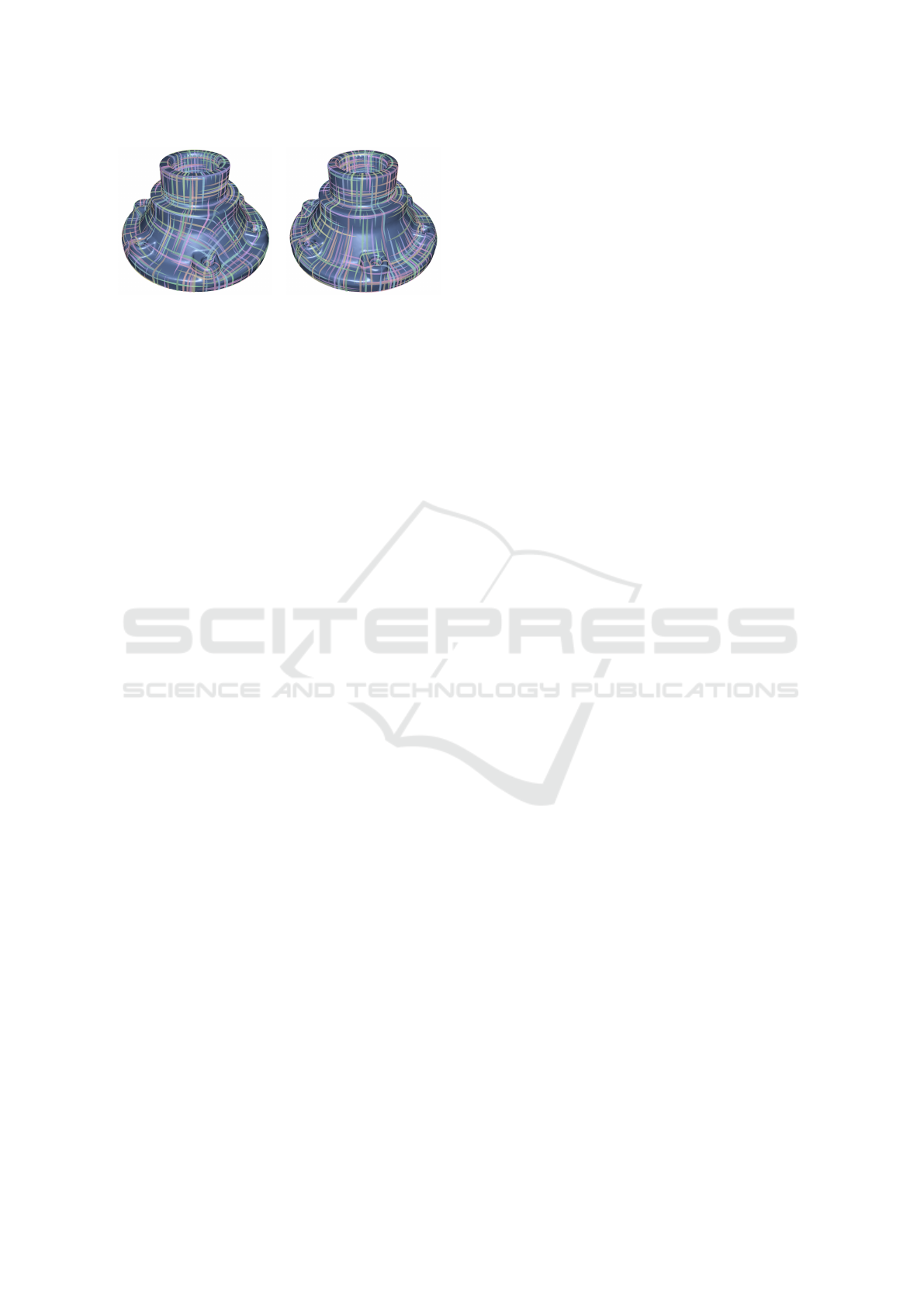
Figure 2: By adding a sparse set of constraints through the
principal directions of vertices that lie on ridges, the orien-
tation field optimisation is better aligned to surface features.
and the neighbour is calculated based on their associ-
ated edge length.
3.7 Extraction
The extraction of the final mesh is done in two stages:
extracting a graph of vertices and their neighbourhood
and then extracting a set of quad-dominant faces from
this neighbourhood. The following three changes
were made to the mesh extraction mechanism.
Minimal Vertex Cluster Size. In (Jakob et al., 2015)
extracted vertices are discarded when the size of their
cluster in the parametrization is smaller than 1/10 of
the average cluster of all extracted vertices to avoid
stray extracted vertices. For most meshes, 1/10 is
appropriate. However, when the extracted mesh has
large faces, the clusters of their vertices may distort
the average such that vertex clusters are discarded that
would still be needed. To give control over this be-
haviour, we added an option to change the fraction of
the cluster size below which vertices are discarded.
Snapping Flat Triangles. When extracting vertices,
the original method (Jakob et al., 2015) may produce
skinny triangles (Botsch and Kobbelt, 2002). These
triangles may cause problems during subsequent pro-
cessing stages of the mesh. As in the original work,
we change their neighbourhood and positioning so
they form a line instead of a triangle.
In (Jakob et al., 2015) three neighbouring vertices
are considered a skinny triangle if the length of any
edge of the triangle is below 30% of the global edge
length scale. However, since the scale is not global
anymore, this threshold does not work and each ex-
tracted vertex needs its own scale. The new scales for
the extracted vertices are based on the scales of the
vertices which contribute to their position in the po-
sition field parametrization. They are computed as a
weighted sum over all scales of contributing vertices,
using the same weights as the computation of the ex-
tracted vertex positions. We define the new threshold
for skinny triangles to be the sum of 10% of each ex-
tracted vertex’ scale. It is equivalent to the original
threshold when all vertices have the same scale.
If a skinny triangle is encountered, the vertex for
which the scale was calculated is moved. If this vertex
is close to one of the other two vertices of the triangle
then these two are merged and their position is aver-
aged. When the vertex to be moved is not close to any
of the other vertices forming the triangle it is moved
so that all three vertices are collinear. Unfortunately,
this simple threshold is sometimes moving vertices
away from feature lines of the reference mesh, which
decreases the quality of the mesh.
To prevent bad snapping, we set the position of
merged vertices to be the position of the vertex with
greater principal curvature instead of computing an
averaged position. Collinear snapping is only per-
formed if the extracted vertex to be moved does not
lie on a feature line (i.e., it has less than two contribut-
ing input feature vertices) or all three vertices of the
extracted triangle lie on a feature line (i.e., more than
one feature vertex).
Creating Quads. When extracting faces, the algo-
rithm of Jakob et al. (Jakob et al., 2015) searches for
polygons in the adjacency graph of the extracted ver-
tices. A face is created if the polygon is a triangle,
a quad or a pentagon. Selecting quads for filling n-
gons follows a greedy scoring system. For an n-gon
v
0
,v
1
,...,v
n−1
, the score is calculated as a sum of dif-
ferences between the four next angles’ and a right an-
gle, starting from i:
score
i
=
3
∑
j=0
|90
◦
− ](v
1
v
2
v
3
)|
where v
1
= v
i+ j (mod n)
, v
2
= v
i+ j+1 (mod n)
, and v
3
=
v
i+ j+2 (mod n)
.
In (Jakob et al., 2015), no reasoning for this scoring is
given and it does not try to find perfect quads as only
the first two angles (i.e. j = 0, j = 1) are part of the
quad.
To favour optimal quads, we use a new scor-
ing system which does not use four consecutive
angles but the four angles of the quad in ques-
tion. We therefore define the score as above but
use the following expressions for the angles: v
1
=
v
i+ j (mod n)
, v
2
= v
i+( j+1 (mod 4)) (mod n)
, and v
3
=
v
i+( j+2 (mod 4)) (mod n)
.
This scoring now fills the space with the most rectan-
gular quad first. Observations on the behaviour sug-
gest that the best quads are also well aligned with the
principal directions and that no additional considera-
tion for this alignment is necessary.
Creating Curvature Adapted Subdivision Control Meshes from Scan Data
153
3.8 Ensuring Manifoldness
Because of the local nature of the position field op-
timisation and the greedy face creation, extracting a
manifold quad-dominant mesh is not always possible.
To remove the non-manifold parts of the mesh, Jakob
et al. perform two passes where faces introducing
non-manifold edges and then all faces surrounding
non-manifold vertices are deleted. However, deleting
affected faces results in holes. We changed the algo-
rithm presented in (Jakob et al., 2015) to repair non-
manifoldness instead of deleting it. Non-manifold
normals (i.e. neighbouring faces with opposite nor-
mals) are not created during the extraction and do not
need to be handled.
Non-manifold Edges. Non-manifold edges can
be detected in the directed edge data-structure (Cam-
pagna et al., 1998) used to represent the extracted
mesh, when the same directed edge is introduced by
two faces. Removal of these edges is done by chang-
ing the affected faces or by removing one face. The
method to repair a non-manifold edge is as follows:
delete all vertices in both faces which are not part of
the non-manifold edge and are adjacent to only one or
two faces in total. If no vertex is deleted, delete one
face as a last resort (if the non-manifold edge is a di-
agonal on one face, delete this face - otherwise delete
a random face). When the deleted vertices leave faces
with 2 or fewer vertices, they are deleted as well.
Non-manifold Vertices. Non-manifold vertices can
be detected by creating a list of all faces adjacent to
the vertex, starting at a random neighbouring face,
traversing the neighbourhood of the vertex and re-
moving all encountered faces off the list. If the vertex
is non-manifold, it has more than one neighbouring
face loop. So, if the list is not empty after all faces
were visited, the vertex is non-manifold. To find all
loops, this loop-search is repeated until all neighbour-
ing faces have been assigned to a face loop. For each
additional face loop, a new vertex is created and all
instances of the non-manifold vertex are positioned to
be the average of all adjacent vertices in their respec-
tive face loop.
While this method removes all non-manifold el-
ements, it cannot guarantee that no holes are cre-
ated, because there are cases where faces cannot be
changed and must be deleted to ensure manifoldness.
Since our goal is a closed mesh, the algorithm de-
scribed in Section 3.7 is used to find and patch poten-
tial holes. To ensure that the hole-filling does not in-
troduce non-manifoldness, one more iteration of non-
manifold clean-up is performed.
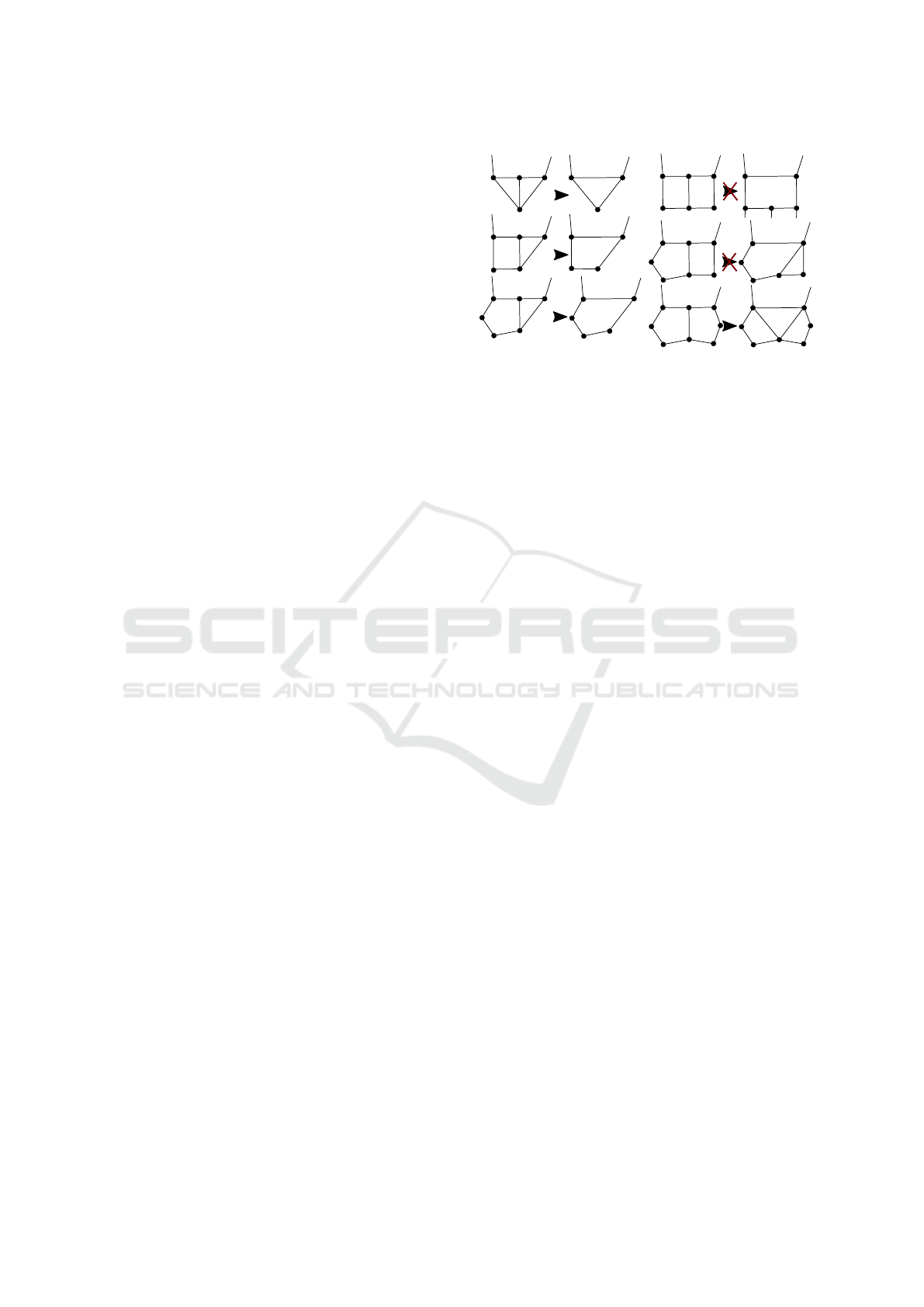
Figure 3: The cases considered in the elimination of T-
junctions in the mesh as described in Section 3.9. Not all
cases improve the quality of the mesh: Combining two
quads (top right) is not feasible because this would intro-
duce more non-quadrilateral faces to the mesh. Combining
a quad and a 5-gon (second right) would create a triangle
and a 5-gon, which is not favourable as well. While two
5-gons are possible in theory, it has not occurred during yet.
3.9 Mesh Post-processing
After the non-manifold clean-up, the extracted mesh
still has potential for improvement. The follow-
ing three additional passes for optimisation are per-
formed.
Eliminating T-junctions. T-junctions in the ex-
tracted mesh induce extraordinary vertices in the sub-
division control mesh. We can avoid T-junctions by
altering the topology of the mesh as shown in Figure
3. To prevent losing detail, the two faces on either side
of the edge ending in a T-junction must lie on similar
planes and their edges adjacent to the T-vertex must
lie, approximately, on a line. For the purposes of this
clean-up, two faces lie on similar planes when their
normals differ by less than five degrees. Two outgo-
ing edges from the T-vertex lie on similar lines when
the angle α between them is 175
◦
< α < 185
◦
. These
angles have shown to be a fitting threshold. Figure 3
shows the different combinations of faces and their
resolved topology. This elimination of T-junctions
tends to reduce the number of non-quads and reduces
the number of extraordinary vertices in the subdivi-
sion control mesh by one.
Feature Aligned Quad Edges. To ensure align-
ment of edges with surface features, two different
approaches are used: The mis-aligned quad face is
split into two triangles along the face diagonal closest
to the feature or the quad face is removed by merg-
ing both endpoints of the diagonal on the feature line
along the middle of the diagonal. Although removal
does not introduce non-quads, it must be done with
caution, because the quad may lie on a high curvature
part of the feature line and removing it could increase
GRAPP 2020 - 15th International Conference on Computer Graphics Theory and Applications
154
the error to the reference mesh. Hence, only quads
where the diagonal has a pair of adjacent edges which
lie on a common line are removed, and all others are
split into two triangles. We consider a pair of out-
going edges from both ends of the diagonal to be on
the same line if, as before, the angle α between the
edges is 175
◦
< α < 185
◦
. This angular threshold was
determined empirically through observations over all
compared meshes.
Finding these quads is a delicate task because
false-positives must be avoided. We used the follow-
ing criteria as a classification of mis-aligned quads:
• The average angle between the orientation field of
both end-vertices and the face diagonal (with 90
◦
rotation symmetry) must be smaller than 15
◦
.
• The angle of the two triangles on both sides of the
diagonal on the feature must be greater than 50
◦
.
• The average largest principal curvature of both
end-vertices of the diagonal must be greater than
the curvature of the other face diagonal.
• The closest face of the reference mesh must be
closer to the middle of the face diagonal than the
middle of the other diagonal.
The first three criteria make sure that only quads
on sharp feature lines are considered. The fourth cri-
teria excludes false-positives where the removal or
split would be performed on the wrong diagonal and
thus worsening the result.
This post-processing improves the feature align-
ment of the extracted mesh. Edges follow the feature
lines again and when a quad is removed, the endpoints
of the diagonal are combined. The outcome of both
approaches of ensuring feature alignment are shown
in Figure 4.
Flat Neighbouring Triangles. We further reduce
the number of non-quad faces in the mesh by merging
neighbouring triangles which lie on a similar plane.
This post-processing is applied before and after elim-
inating T-junctions and aligning edges with features.
Two triangles are considered lying on a similar plane
based on the same threshold as in Section 3.9.
3.10 Smoothing
The position field optimisation does not always pro-
duce perfect quads. Especially in areas where large
edge lengths meet short edge lengths, some quads
might be very distorted. To improve the quality of dis-
torted quads without losing detail, tangential smooth-
ing is performed. New vertex points are computed
by averaging over all neighbours in a 1-ring neigh-
bourhood and then projecting them onto the tangen-
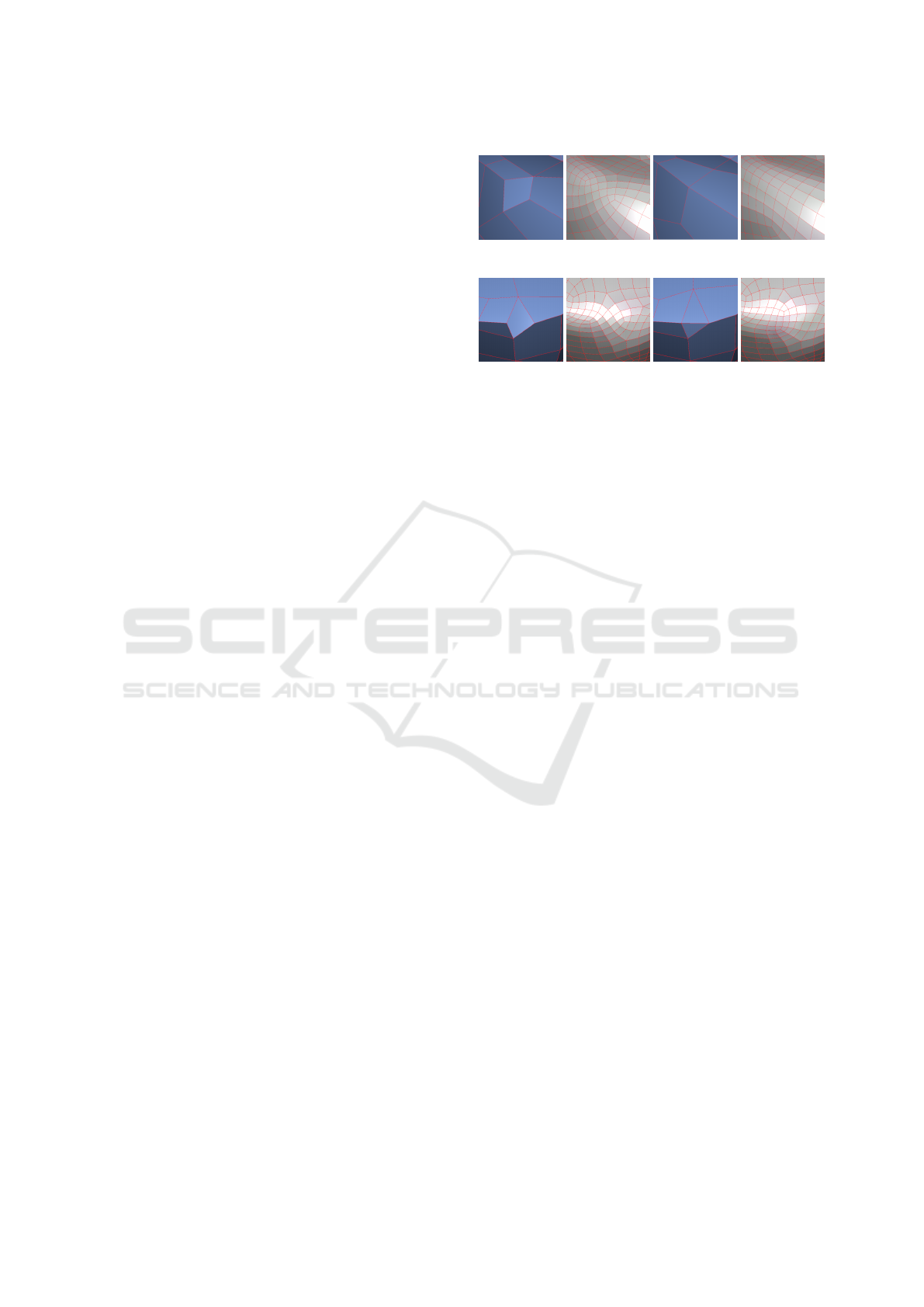
(a) Quad to be removed (b) After quad removal
(c) Quad to be split (d) After quad split
Figure 4: The meshes and their corresponding subdivision
meshes are shown before and after post-processing to avoid
mis-aligned edges. Figures (a) and (c) show meshes with
mis-aligned edges together with their corresponding subdi-
vision mesh. Figures (b) and (d) show the meshes together
with their subdivision meshes after post-processing. The
ridge lines are kept intact by removing or splitting the quads
as described in Section 3.9.
tial plane of the original vertex. To preserve the fea-
tures of the mesh, vertices are not smoothed when
the largest angle between the normals of their neigh-
bouring faces is greater than 50
◦
. Three iterations of
smoothing are able to restore distorted quads while
largely preserving the difference in edge length.
3.11 Subdivision Control Mesh
The next step is creating a Catmull-Clark subdivision
control mesh from the extracted quad-dominant mesh.
A subdivision control mesh is created via iteratively
moving the vertices of the quad-dominant mesh along
their normal until the limit point closely approximates
the input mesh as described previously in (Thaller
et al., 2016). The algorithm to derive a subdivision
control mesh from a polygon mesh is as follows:
mesh ← output of instant meshes
while Less than 20 iterations do
for all vertices ∈ mesh do
LimitPoint ← limit point of vertex
I ← intersection of reference mesh and
Ray[LimitPoint, normal]
NewVertexPos ← vertex + (I − LimitPoint)
end for
if max
v∈mesh
|NewVertexPos − OldVertexPos| < ε
then
break
end if
mesh ← all NewVertexPos
end while
The algorithm stops either after 20 iterations or when
Creating Curvature Adapted Subdivision Control Meshes from Scan Data
155
the maximum distance between old and new posi-
tions for vertices are below a threshold ε. Our ε is
10
−4
× the greatest dimension of the reference meshes
bounding box.
To apply this algorithm, the limit points of the ex-
tracted mesh need to be calculated. Catmull-Clark
subdivision surfaces correspond to bi-cubic B-splines
in the regular region. In non-regular regions, for ver-
tices with valences not equal to four, (Halstead et al.,
1993) have derived a linear combination to compute
the limit points from the control points.
4 RESULTS
The meshes resulting from our work are able to rep-
resent reference meshes up to a user-defined desired
error, with an emphasis on distributing vertices so that
high frequency details are preserved.
A change in density in quad meshes leads to ver-
tices with a valence different to four or to the intro-
duction of non-quads. Therefore, our resulting quad-
dominant meshes have more extraordinary vertices
compared with other approaches. They have uniform
quads in regions of similar curvature of the reference
mesh and adapt to changes in curvature with non-
quads or EVs. The number of EVs and non-quads of
our method depends on the number of transitions be-
tween low and high curvature regions because quad-
dominant meshes need non-quads or EVs to make the
corresponding transition of edge lengths.
Most isotropic approaches aim for pure quad or
quad-dominant meshes while trying to minimise the
number of EVs. This limits their abilities to adapt
to curvature. Compared to our method, the isotropic
meshes of Jakob et al. (Jakob et al., 2015) are more
regular with fewer EVs and non-quads, and have
quads with better quality. However, they are less
dense in high curvature regions and thus cannot rep-
resent high frequency detail as well (c.f. Figure 5).
Additionally, due to the dependence on curvature es-
timation, our approach is slower, but still interactive
(timings with 16GB RAM, Intel i7-4930K CPU):
#Input Vertices Jakob et al. (ms) Our work(ms)
14000 500 1300
50000 850 2700
100000 1300 4600
To compare the original work of Jakob et al. and
our contribution, we extracted meshes with a similar
number of vertices through both approaches. We used
the default setting for the original work but changed
the desired number of extracted vertices to match our
resulting meshes. Since the algorithm can only be
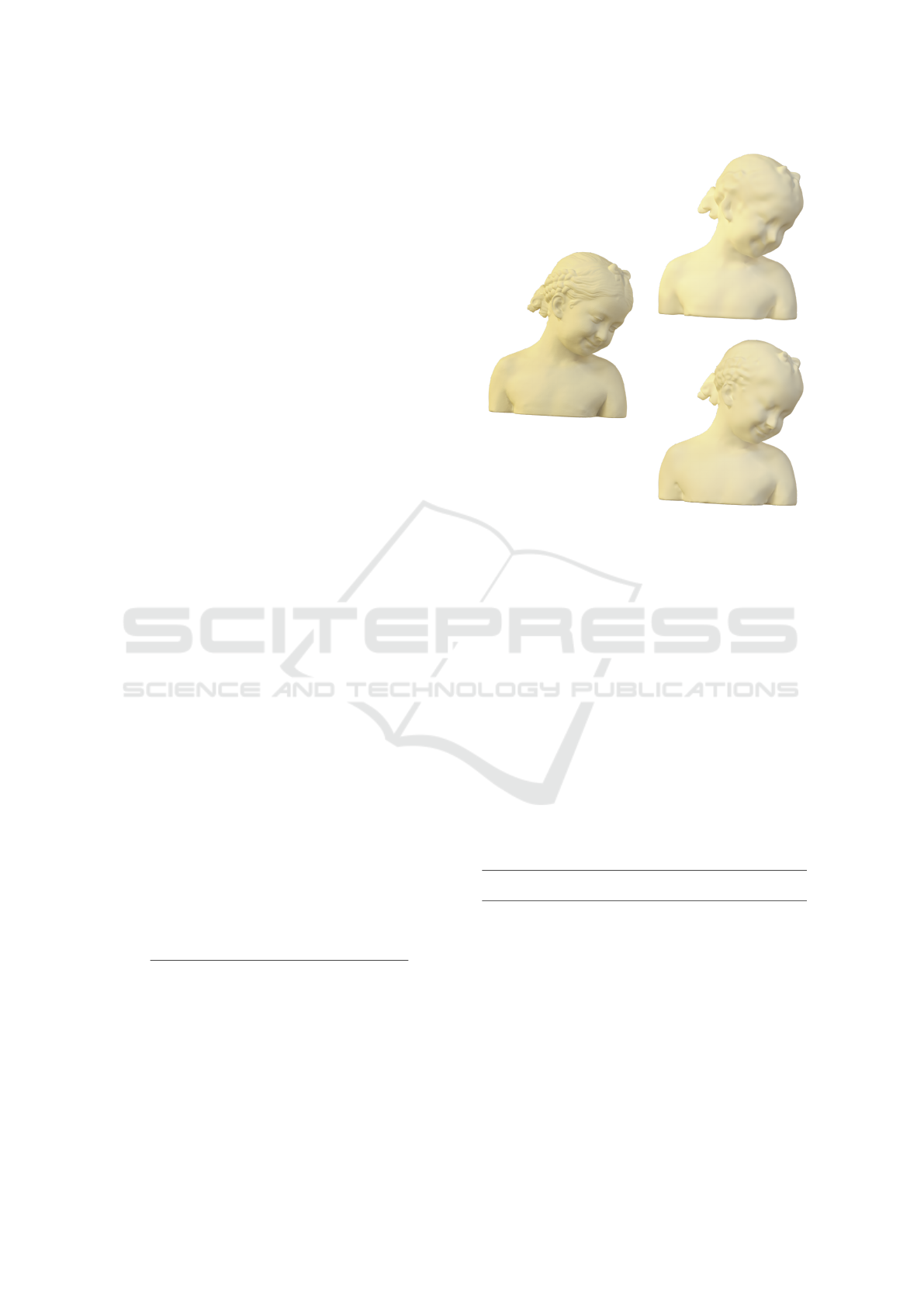
Our work:
Jakob et al.:
2108 vertices
96.2% reduction
2076 vertices
96.3% reduction
Mesh Name: Bimba
Figure 5: Comparison of subdivision surfaces for the origi-
nal work (top) and our method (bottom) with a high density
and the rendered original scan data (left).
set to approximate a number of vertices, we cannot
compute the exact same number of vertices for both
approaches. Both types of meshes were converted
to subdivision control meshes. A visual compari-
son of the resulting subdivision surfaces demonstrates
clearly how the algorithm presented in this paper is
able to capture high frequency details present in the
original data with a similar number of vertices.
To quantify the improvement, we employ a
number of error metrics to compare subdivision
surface derived using the approach presented in this
paper to those derived from quad meshes using Jakob
et al.’s approach. Averaged over all meshes compared
in this paper, the following error can be observed:
Error Metric EV’s
Hausdorff
Distance
Avg. Quad
Quality
Avg. Face
Centroid Dist.
Jakob et al. 0.28% 0.468 0.489 0.122
Our algorithm 0.89% 0.463 1.291 0.115
% Difference +246.01% -2.90% +180.79% -6.06%
Here, the average quad quality is an adapted quad
quality measure taken from (Marinov and Kobbelt,
2006) and the average face centroid distance to
the reference mesh is used to avoid large quads in
detailed regions. The adaptation of the quad quality
measure comes from omitting the deviation from a
square, since our goal is not a perfect isotropic mesh.
The introduced curvature-dependent vertex densi-
ties improve the Hausdorff distances between limit
surface and reference mesh. It also shows how the
focus on adaptive edge length increases the number
GRAPP 2020 - 15th International Conference on Computer Graphics Theory and Applications
156
Our work:
Jakob et al.:
723 vertices
98.5% reduction
706 vertices
98.5% reduction
Mesh Name: Igea
High Error
Low Error
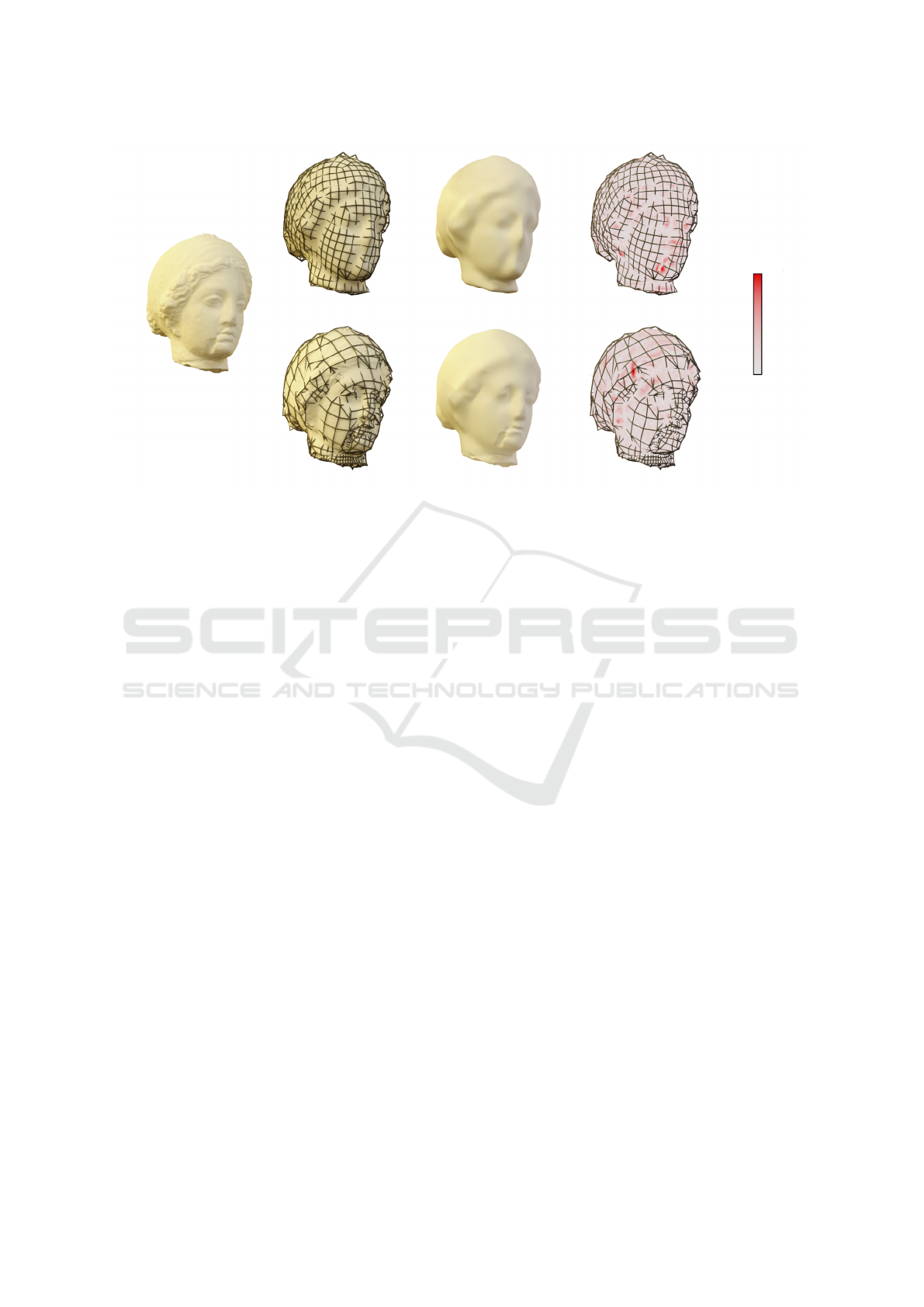
Figure 6: On the left is the rendered input mesh resulting from scan capture. 2nd from left: The subdivision control mesh
generated from the scan data. The limit surface derived from control mesh is shown 3rd from left. On the right we used colour
to highlight the error between the scan data and the subdivision limit surface. Our algorithm creates a control mesh which is
dense in regions where it is required to capture fine detail, but coarse in regions of low curvature (bottom row). The resulting
limit surface captures high frequency features at a considerably higher precision opposed to the original approach by Jakob
et al., who are more concerned with regularity of the underlying mesh. Despite a similar number of vertices, our algorithm
captures the scar around the mouth quite well, while using a coarse grid in regions with less detail.
of extraordinary vertices and deteriorates quad qual-
ity. Additionally, the proposed algorithm struggles
when two very flat areas meet at a sharp crease. The
problem arises from the very concentrated high cur-
vature region of the sharp crease being surrounded by
nearly zero curvature. When the disparity between
large edge lengths and small edge lengths is too sud-
den, the position field optimisation may not produce
optimal results. To tackle this, however, curvature can
either be smoothed stronger for more gradual curva-
ture changes, or the desired error can be set lower to
create smaller quads overall.
Figure 6 and Figure 7 compare the different
meshes and errors between the original and our ap-
proach. They show the improved accuracy in detailed
regions and more irregular meshes that our curvature
adapted edge lengths produce, when compared to the
isotropic approach in (Jakob et al., 2015). Figure 8
compares the results of both approaches for a variety
of meshes. The most notable differences are in re-
gions with fine detail.
All our additional methods and many options for
the behaviour of the algorithms are added to the soft-
ware created in (Jakob et al., 2015). With the embed-
ded batch mode, a user may extract quad-dominant or
subdivision control meshes quickly based on our set
of default options. Because of the variety of options,
it is also possible to find a set of parameter setting to
obtain improved results for specific meshes. Because
the extraction is fast and initialisation is random, try-
ing different options to find good solutions is easy.
5 CONCLUSION
We have created an adaptive quad-dominant meshing
method with a focus on curvature-dependent density
to accurately capture high frequency detail in the orig-
inal data. A subsequent conversion of the extracted
quad meshes to subdivision control meshes yields
subdivision surfaces that faithfully describe even de-
tailed features of the original shape. Possible defects
in the parametrisation have been addressed through
post-processing steps. Our algorithm presented in this
paper enables the creation of coarse subdivision con-
trol meshes with corresponding subdivision limit sur-
faces which precisely model arbitrary shapes with a
low number of vertices, while still accurately repre-
senting the reference shape, by offering higher den-
sity of the control mesh in regions with detailed fea-
tures. The trade-off, however, is higher irregularity of
the derived subdivision control mesh.
The design is very flexible and may be adapted
to more specialised applications. Our focus was on
an automated process that is able to produce satisfy-
ing results for a variety of inputs. Further work may
Creating Curvature Adapted Subdivision Control Meshes from Scan Data
157
Our work:
Jakob et al.:
2283 vertices
96.1% reduction
2358 vertices
95.9% reduction
Mesh Name: Rampant
High Error
Low Error
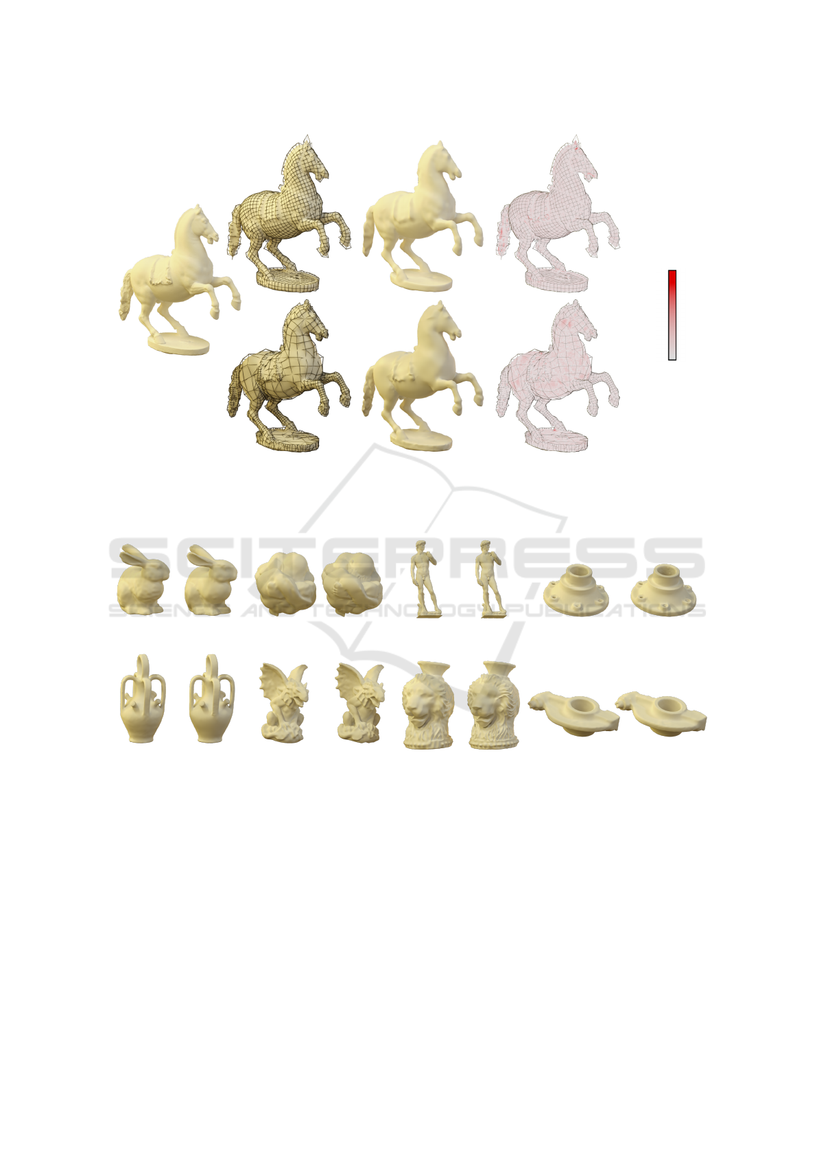
Figure 7: Same setup as Figure 6. We can see that the high frequency areas are better preserved with out approach (bottom),
however, low frequency areas around the neck and behind the saddle lose some detail as their curvature is too low. This shows
how our method distributes the expected error more evenly over the mesh, while still maintaining a low number of vertices.
Jakob et al.
Our work
1406 vertices
1483 vertices
Omotondo
Jakob et al.
Our work
2062 vertices
1991 vertices
Stanford Bunny
Jakob et al.
Our work
4349 vertices
4249 vertices
David
Jakob et al.
Our work
4202 vertices
4176 vertices
Carter
Jakob et al.
Our work
1736 vertices 1666 vertices
Rocker Arm
Jakob et al.
Our work
2893 vertices 2995 vertices
Vase Lion
Jakob et al.
Our work
2567 vertices 2400 vertices
Botijo
Jakob et al.
Our work
2320 vertices 2404 vertices
Gargoyle
Figure 8: An overview over a variety of resulting subdivision meshed for both approaches and the mesh names. Vertex
numbers represent the extracted control meshes that were used to generate the subdivision meshes. All input meshes were
taken from the supplementary material of (Jakob et al., 2015).
include more post-processing to ensure that the ex-
tracted meshes fulfil the demands of more specific
applications, more specialised settings for a subset
of meshes or different constraints on the parametri-
sation.
REFERENCES
Alliez, P., Cohen-Steiner, D., Devillers, O., L
´
evy, B., and
Desbrun, M. (2003). Anisotropic polygonal remesh-
ing. ACM Transactions on Graphics, 22(3):485.
Bommes, D., Campen, M., Ebke, H.-C., Alliez, P., and
Kobbelt, L. (2013a). Integer-grid maps for reli-
able quad meshing. ACM Transactions on Graphics,
32(4):1.
GRAPP 2020 - 15th International Conference on Computer Graphics Theory and Applications
158

Bommes, D., L
´
evy, B., Pietroni, N., Puppo, E., Silva, C.,
Tarini, M., and Zorin, D. (2013b). Quad-mesh gener-
ation and processing: A survey. Computer Graphics
Forum, 32(6):51–76.
Bommes, D., Zimmer, H., and Kobbelt, L. (2009). Mixed-
integer quadrangulation. ACM Transactions on
Graphics, 28(3):1.
Botsch, M. and Kobbelt, L. (2002). A robust procedure
to eliminate degenerate faces from triangle meshes.
Proc. of Vision, Modeling, and Visualization 01.
Campagna, S., Kobbelt, L., and Seidel, H.-P. (1998). Di-
rected Edges - A Scalable Representation for Triangle
Meshes. Journal of Graphics Tools, 3(4):1–11.
Campen, M., Bommes, D., and Kobbelt, L. (2012). Dual
loops meshing. ACM Transactions on Graphics,
31(4):1–11.
Dong, S., Bremer, P.-T., Garland, M., Pascucci, V., and
Hart, J. C. (2006). Spectral surface quadrangulation.
ACM Transactions on Graphics, 25(3):1057.
Dong, S., Kircher, S., and Garland, M. (2005). Har-
monic functions for quadrilateral remeshing of arbi-
trary manifolds. Computer Aided Geometric Design,
22(5):392–423.
Gatzke, T. D. and Grimm, C. M. (2006). Estimating Curva-
ture on Triangular Meshes. International Journal of
Shape Modeling, 12(01):1–28.
Goldfeather, J. and Interrante, V. (2004). A novel cubic-
order algorithm for approximating principal direction
vectors. ACM Transactions on Graphics, 23(1):45–
63.
Halstead, M., Kass, M., and DeRose, T. D. (1993). Ef-
ficient, fair interpolation using Catmull-Clark sur-
faces. In Proceedings of the 20th annual conference
on Computer graphics and interactive techniques -
SIGGRAPH ’93, SIGGRAPH ’93, pages 35–44, New
York, NY, USA. ACM.
Hormann, K. and Greiner, G. (2000). Quadrilateral remesh-
ing. In Proceedings of Vision, Modeling and Vizual-
ization, 2000, pages 153–162.
Jakob, W., Tarini, M., Panozzo, D., and Sorkine-Hornung,
O. (2015). Instant field-aligned meshes. ACM Trans-
actions on Graphics, 34(6):1–15.
K
¨
alberer, F., Nieser, M., and Polthier, K. (2007). Quad-
Cover - Surface Parameterization using Branched
Coverings. Computer Graphics Forum, 26(3):375–
384.
Kovacs, D., Myles, A., and Zorin, D. (2011). Anisotropic
quadrangulation. Computer Aided Geometric Design,
28(8):449–462.
Lai, Y. K., Kobbelt, L., and Hu, S. M. (2010). Feature
aligned quad dominant remeshing using iterative local
updates. CAD Computer Aided Design, 42(2):109–
117.
Liu, Y., Xu, W., Wang, J., Zhu, L., Guo, B., Chen, F., and
Wang, G. (2011). General planar quadrilateral mesh
design using conjugate direction field. ACM Transac-
tions on Graphics, 30(6):1.
Ljung, P., Kr
¨
uger, J., Groller, E., Hadwiger, M., Hansen,
C. D., and Ynnerman, A. (2016). State of the Art
in Transfer Functions for Direct Volume Rendering.
Computer Graphics Forum, 35(3):669–691.
Marinov, M. and Kobbelt, L. (2004). Direct anisotropic
quad-dominant remeshing. In Proceedings - Pacific
Conference on Computer Graphics and Applications,
PG ’04, pages 207–216, Washington, DC, USA. IEEE
Computer Society.
Marinov, M. and Kobbelt, L. (2006). A robust two-step
procedure for quad-dominant remeshing. Computer
Graphics Forum, 25(3):537–546.
Myles, A., Pietroni, N., Kovacs, D., and Zorin, D. (2010).
Feature-aligned T-meshes. ACM SIGGRAPH 2010
papers on - SIGGRAPH ’10, (July 2010):1.
Petitjean, S. (2002). A survey of methods for recovering
quadrics in triangle meshes. ACM Computing Surveys,
34(2):211–262.
Ray, N., Li, W. C., L
´
evy, B., Sheffer, A., and Alliez, P.
(2006). Periodic global parameterization. ACM Trans-
actions on Graphics, 25(4):1460–1485.
Rugis, J. and Klette, R. (2006). A scale invariant sur-
face curvature estimator. Lecture Notes in Computer
Science (including subseries Lecture Notes in Artifi-
cial Intelligence and Lecture Notes in Bioinformatics),
4319 LNCS:138–147.
Thaller, W., Augsd
¨
orfer, U., and Fellner, D. W. (2016).
Procedural mesh features applied to subdivision sur-
faces using graph grammars. Computers and Graph-
ics (Pergamon), 58:184–192.
Tong, Y., Alliez, P., Cohen-Steiner, D., and Desbrun, M.
(2006). Designing Quadrangulations with Discrete
Harmonic Forms. In Eurographics Symposium on Ge-
ometry Processing, SGP ’06, pages 201–210, Aire-la-
Ville, Switzerland, Switzerland. Eurographics Associ-
ation.
Zhang, M., Huang, J., Liu, X., and Bao, H. (2010). A wave-
based anisotropic quadrangulation method. ACM
Transactions on Graphics, 29(4):1.
Zhang, M., Huang, J., Liu, X., and Bao, H. (2013).
A divide-and-conquer approach to quad remeshing.
IEEE Transactions on Visualization and Computer
Graphics, 19(6):941–952.
Creating Curvature Adapted Subdivision Control Meshes from Scan Data
159
