Visual Descriptor Learning from Monocular Video
Umashankar Deekshith
a
, Nishit Gajjar
b
, Max Schwarz
c
and Sven Behnke
d
Autonomous Intelligent Systems Group of University of Bonn, Germany
Keywords:
Dense Correspondence, Deep Learning, Pixel Descriptors.
Abstract:
Correspondence estimation is one of the most widely researched and yet only partially solved area of computer
vision with many applications in tracking, mapping, recognition of objects and environment. In this paper,
we propose a novel way to estimate dense correspondence on an RGB image where visual descriptors are
learned from video examples by training a fully convolutional network. Most deep learning methods solve
this by training the network with a large set of expensive labeled data or perform labeling through strong
3D generative models using RGB-D videos. Our method learns from RGB videos using contrastive loss,
where relative labeling is estimated from optical flow. We demonstrate the functionality in a quantitative
analysis on rendered videos, where ground truth information is available. Not only does the method perform
well on test data with the same background, it also generalizes to situations with a new background. The
descriptors learned are unique and the representations determined by the network are global. We further show
the applicability of the method to real-world videos.
1 INTRODUCTION
Many of the problems in computer vision, like 3D
reconstruction, visual odometry, simultaneous local-
ization and mapping (SLAM), object recognition, de-
pend on the underlying problem of image correspon-
dence (see Fig. 1). Correspondence methods based on
sparse visual descriptors like SIFT (Lowe, 2004) have
been shown to be useful for applications like cam-
era calibration, panorama stitching and even robot
localization. However, SIFT and similar hand de-
signed features require a textured image. They per-
form poorly for images or scenes which lack sufficient
texture. In such situations, dense feature extractors
are better suited than sparse keypoint-based methods.
With the advancement in deep learning in recent
years, the general trend is that neural networks can be
trained to outperform hand designed feature methods
for any function using sufficient training data. How-
ever, supervised training approaches require signifi-
cant effort because they require labeled training data.
Therefore, it is useful to have a way to train the model
in a self-supervised fashion, where the training labels
are created automatically.
a
https://orcid.org/0000-0002-0341-5768
b
https://orcid.org/0000-0001-7610-797X
c
https://orcid.org/0000-0002-9942-6604
d
https://orcid.org/0000-0002-5040-7525
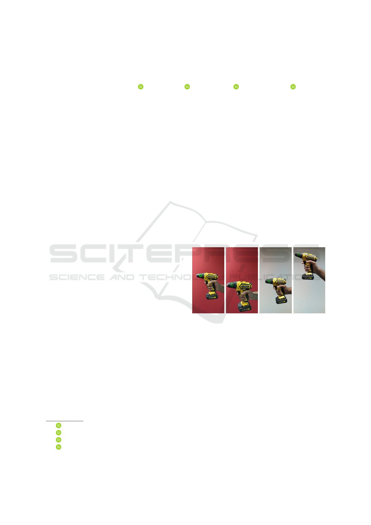
Figure 1: Point tracking using the learned descriptors in
monocular video. Two different backgrounds are shown to
represent the network’s capability to generate global corre-
spondences. A square patch of 25 pixels are selected (left)
and the nearest neighbor for those pixels based on the pixel
representation is shown for the other images.
In their work, (Schmidt et al., 2017) and (Flo-
rence et al., 2018) have shown approaches for self-
supervised visual descriptor learning using raw RGB-
D sequence of images. Their approach shows that it
is possible to generate dense descriptors for an ob-
ject or a complete scene and that these descriptors are
consistent across videos with different backgrounds
and camera alignments. The dense descriptors are
learned using contrastive loss (Hadsell et al., 2006).
The method unlocks a huge potential for robot ma-
nipulation, navigation, and self learning of the envi-
ronment. However, for obtaining the required corre-
spondence information for training, the authors rely
444
Deekshith, U., Gajjar, N., Schwarz, M. and Behnke, S.
Visual Descriptor Learning from Monocular Video.
DOI: 10.5220/0008989304440451
In Proceedings of the 15th International Joint Conference on Computer Vision, Imaging and Computer Graphics Theory and Applications (VISIGRAPP 2020) - Volume 5: VISAPP, pages
444-451
ISBN: 978-989-758-402-2; ISSN: 2184-4321
Copyright
c
2022 by SCITEPRESS – Science and Technology Publications, Lda. All rights reserved
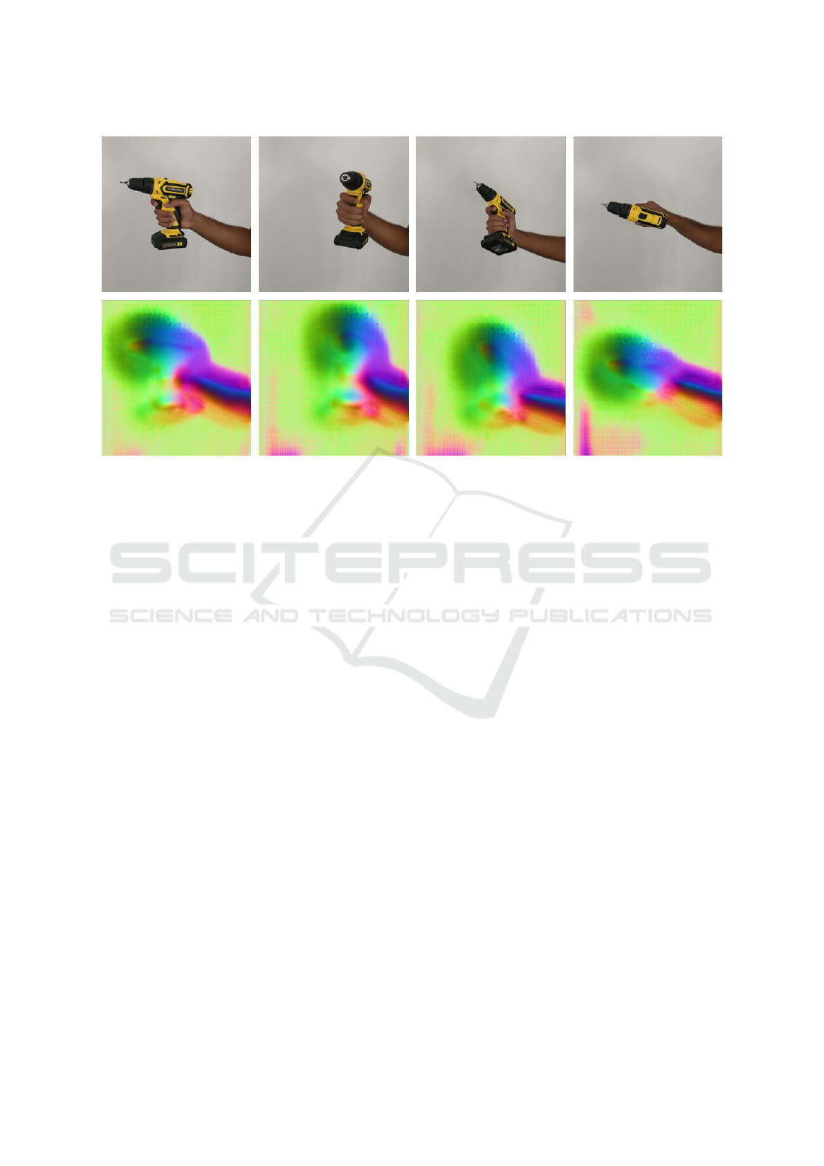
Figure 2: Learned dense object descriptors. Top: Stills from a monocular video demonstrating full 6D movement of the object.
Bottom: Normalized output of the trained network where each pixel is represented uniquely, visualized as an RGB image.
The objects were captured in different places under different lighting conditions, viewpoints giving the object a geometric
transformation in a 3D space. It can be seen here that the descriptor generated is independent of these effects. This video
sequence has not been seen during training.
on 3D reconstruction from RGB-D sensors. This lim-
its the applicability of their method (i.e. shiny and
transparent objects cannot be learned).
Every day a large quantity of videos are generated
from basic point and shoot cameras. Our aim is to
learn the visual descriptors from an RGB video with-
out any additional information. We follow a similar
approach to (Schmidt et al., 2017) by implementing
a self-supervised visual descriptor learning network
which learns dense object descriptors (see Fig. 2). In-
stead of the depth map, we rely on the movement
of the object of interest. To find an alternate way
of self learning the pixel correspondences, we turn
to available optical flow methods. The traditional
dense optical flow method of (Farneb
¨
ack, 2000) and
new deep learning based optical flow methods (Sun
et al., 2017; Ilg et al., 2017) provide the information
which is the basis of our approach to generate self-
supervised training data. Optical flow gives us a map-
ping of pixel correspondences within a sequence of
images. Loosely speaking, our method turns relative
correspondence from optical flow into absolute corre-
spondence using our learned descriptors.
To focus the descriptor learning on the object of
interest, we employ a generic foreground segmenta-
tion method (Chen et al., 2014), which provides a
foreground object mask. We use this foreground mask
to limit the learning of meaningful visual descriptors
for the foreground object, such that these descriptors
are as far apart in descriptor space as possible.
In this work, we show that it is possible to learn
visual descriptors for monocular images through self-
supervised learning by training them using contrastive
loss for images labeled from optical flow information.
We further demonstrate applicability in experiments
on synthetic and real data.
2 RELATED WORK
Traditionally, dense correspondence estimation algo-
rithms were of two kinds. One with focus on learning
generative models with strong priors (Hinton et al.,
1995), (Sudderth et al., 2005). These algorithms were
designed to capture similar occurrence of features.
Another set of algorithms use hand-engineered meth-
ods. For example, SIFT or HOG performs cluster-
ing over training data to discover the feature classes
(Sivic et al., 2005), (C. Russell et al., 2006). Re-
cently, the advances in deep learning and their abil-
ity to reliably capture high dimensional features di-
rectly from the data has made a lot of progress in
correspondence estimation, outperforming the tradi-
tional methods. (Taylor et al., 2012) have proposed
a method where a regression forest is used to predict
dense correspondence between image pixels and ver-
Visual Descriptor Learning from Monocular Video
445

tices of an articulated mesh model. Similarly, (Shot-
ton et al., 2013) use a random forest given only a sin-
gle acquired image, to deduce the pose of an RGB-D
camera with respect to a known 3D scene. (Brach-
mann et al., 2014) jointly train an objective over both
3D object coordinates and object class labeling to de-
termine to address the problem of estimating the 6D
Pose of specific objects from a single RGB-D im-
age. Semantic segmentation of images as presented
by (Long et al., 2014; Hariharan et al., 2015) use neu-
ral network that produce dense correspondence of im-
ages. (G
¨
uler et al., 2018) propose a method to estab-
lish dense correspondence between RGB image and
surface based representation of human body. All of
these methods rely on labeled data. To avoid the ex-
pensive labeling process, we use relative labels for
pixels generated before training with minimum com-
putation and no human intervention.
Relative labeling has been in use for various appli-
cations. (Wang et al., 2014) introduced a multi-scale
network with triplet sampling algorithm that learns a
fine-grained image similarity model directly from im-
ages. For image retrieval using deep hashing, (Zhang
et al., 2015) trained a deep CNN where discrimina-
tive image features and hash functions are simulta-
neously optimized using max-margin loss on triplet
units. However, these methods also require labeled
data. (Wang and Gupta, 2015) propose a method
for image patch detection where they employ rela-
tive labeling for data points. Here they try to track
patches in videos where two patches connected by
a track should have similar visual representation and
have closer distance in deep feature space and hence
be able to differentiate it from a third patch. In con-
trast, our method works on pixel level and is thus able
to provide fine-grained correspondence. Also, their
work does not focus on representing a specific patch
distinctively and so it is not clear if a correspondence
generated for a pixel is consistent across different sce-
narios for an object.
Our work makes use of optical flow estimation
(Fischer et al., 2015; Janai et al., 2018; Sun et al.,
2017; Ilg et al., 2017), which has made significant
progress through deep learning. While these ap-
proaches can obviously be used to estimate corre-
spondences for short time frames, our work is applica-
ble for larger geometric transformation, environment
with more light variance and occlusion. Of course, a
better optical flow estimate during training improves
results in our method.
Contrastive loss for dense correspondence has
been used by (Schmidt et al., 2017) where they have
used relative labeling to train a fully convolutional
network. The idea presented by them is for the de-
scriptor to be encoded with the identity of the point
that projects onto the pixel so that it is invariant to
lighting, viewpoint, deformation and any other vari-
able other than the identity of the surface that gener-
ated the observation. (Florence et al., 2018) train the
network for single-object and multi-object descriptors
using a modified pixel-wise contrastive loss function
which (similar to (Schmidt et al., 2017)) minimizes
the feature distance between the matching pixels and
pushes that of non-matching pixels to be at least a
configurable threshold away from each other. Their
aim is to train a robotic arm to generate training data
consisting of objects of interests and then training a
FCN network to distinctively identify different parts
of the same object and multiple objects. In these
methods, an RGB-D video is used and a strong 3D
generative model is used to automatically label cor-
respondences. In absence of the depth information, a
dense optical flow between subsequent frames of an
RGB video can provide the correlation between pix-
els in different frames. For image segmentation to se-
lect the dominant object in the scene, we refer to the
solution given by (Chen et al., 2014) and (Jia et al.,
2014).
3 METHOD
Our aim is to train a visual descriptor network us-
ing an RGB video to get a non-linear function which
can translate an RGB image R
W xHx3
to a descriptor
image R
W xHxD
. In the absence of geometry infor-
mation, two problems need to be solved: The ob-
ject of interest needs to be segmented for training and
pixel correspondences need to be determined. To seg-
ment the object of interest from the scene, we refer
to the off the shelf solution provided by (Chen et al.,
2014). It provides us with a pre-trained network built
on Caffe (Jia et al., 2014) from which masks can be
generated for the dominant object in the scene. To
obtain pixel correspondences we use a dense optical
flow between subsequent frames of an RGB video.
The network architecture and loss function used
for training are as explained below:
3.1 Network Architecture
A fully convolution network (FCN) architecture is
used where the network has 34 layered ResNet(He
et al., 2016) as the encoder block and 6 deconvolu-
tional layers as the decoder block, with ReLU as the
activation function. ResNet used is pre-trained on Im-
ageNet (Deng et al., 2009) data-set. The input has
the size H×W ×3 and the output layer has the size
VISAPP 2020 - 15th International Conference on Computer Vision Theory and Applications
446
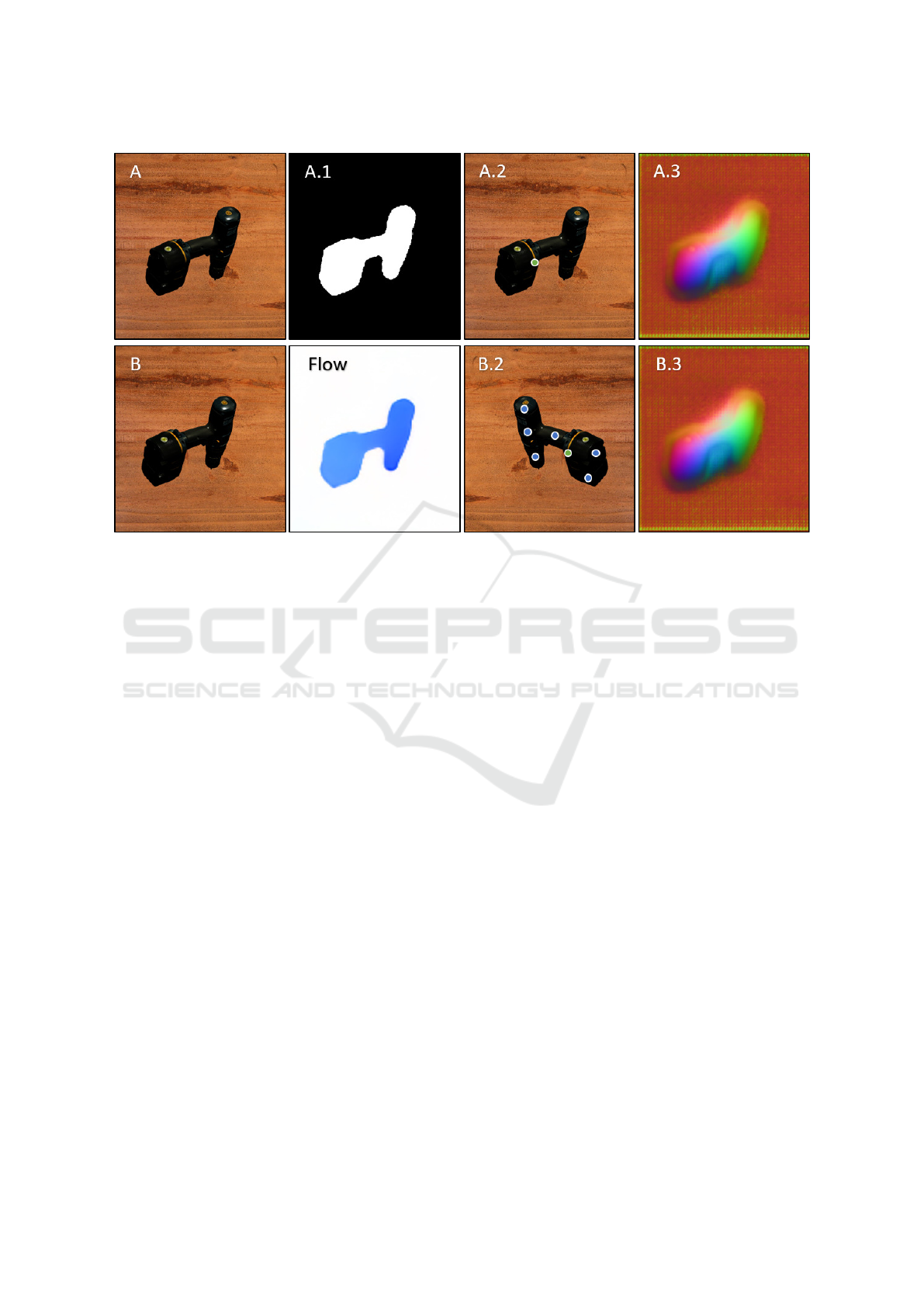
Figure 3: Training process. Images A and B are consecutive frames taken from an input video. A.1: Dominant object mask
generated for segmentation of image A. Flow: Optical flow between images A and B, represented as an RGB image. This
is used for performing automatic labelling of images where pixel movement for every pixel in Image A is represented by
the calculated optical flow. A.2: Training input with a randomly selected reference point (green). B.2: Horizontally flipped
version of image B. Note the corresponding reference point (green), which is calculated using the optical flow offset. The
reference point pair is used as a positive example for contrastive loss. Additional negative samples for the green reference
point in A.2 are marked in blue. A.3, B.3: Learned descriptors for images A and B.
H×W ×D, where D is the descriptor size. The net-
work also has skip connections to retain information
from earlier layers, and L2 normalization at the out-
put.
3.2 Loss Function
A modified version of pixelwise contrastive loss
(Hadsell et al., 2006), as has been used by (Florence
et al., 2018), is used for training. The corresponding
pixel pair determined using the optical flow is consid-
ered as a positive example and the network is trained
to reduce the L2 distance between their descriptors.
The negative pixel pair samples are selected by ran-
domly sampling the pixels from the foreground ob-
ject, where the previously generated mask helps in
limiting the sampling domain to just the object of in-
terest. The negative samples are expected to be at
least m distance away. We thus define the loss func-
tion
L(A, B, u
a
, u
b
, O
A→B
) =
D
AB
(u
a
, u
b
)
2
if O
A→B
(u
a
) = u
b
,
max(0, M − D
AB
(u
a
, u
b
))
2
otherwise.
(1)
where O
A→B
is the optical flow mapping of pixels
from image A to B, M is a margin and D
AB
(u
a
, u
b
)
is the distance metric between the descriptor of image
A at pixel u
a
and the descriptor of image B at pixel u
b
as defined by
D
AB
(u
a
, u
b
) = || f
A
(u
a
) − f
B
(u
b
)||
2
(2)
with the computed descriptor images f
A
and f
B
.
3.3 Training
For training the descriptor space for a particular ob-
ject, an RGB video of the object is used. Masks are
generated for each image by the pre-trained DeepLab
network (Chen et al., 2014) to segment the im-
age into the foreground and background. Two sub-
sequent frames are extracted from the video, and
dense optical flow is calculated using Farneback’s
method (Farneb
¨
ack, 2000) after applying the mask
(see Fig. 3). We also used the improvements in op-
tical flow estimation using Flownet2 (Ilg et al., 2017)
where we generated the optical flow through pre-
trained networks (Reda et al., 2017) for our data-set
and observed that an improvement in optical flow de-
termination does indeed help us in a better correspon-
dence estimation.
Visual Descriptor Learning from Monocular Video
447
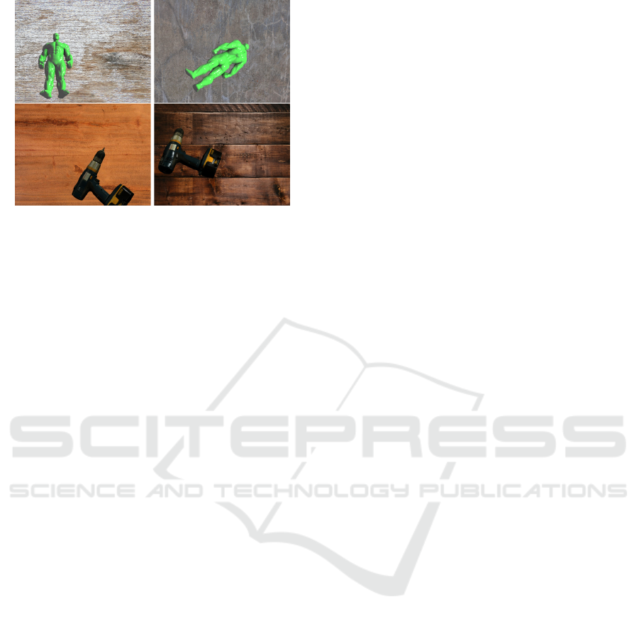
Figure 4: Synthetic images used for experiments. Top row:
Hulk figure, Bottom row: Drill. In both cases, we render
videos with two different background images.
The pair of frames are passed through the FCN
and their outputs along with the optical flow map
are used to calculate the pixel-wise contrastive loss.
Since there are millions of pixels in an image, ’pixel
pair’ sampling needs to be done to increase the speed
of training. For this, only the pixels on the object
of interest are taken into consideration. To select
the pixel pair, the pixel movement is measured us-
ing the optical flow information. As shown in figure
7, once the pixels are sampled from image A, corre-
sponding pixels in image B are found using the op-
tical flow map and these become the pixel matches.
For each sampled pixel from image A, a number of
non-match pixels are sampled uniformly at random
from the object in image B. These create the pixel
non-matches. We experimented with the number of
positive pixel matches in the range of 1000 to 10000
matches and observed that for us, 2000-3000 posi-
tive pixel matches worked the best for us and this
was used for the results. For each match 100-150
non-match pairs are considered. The loss function
is applied and averaged over the number of matches
and non-matches and then the loss is backpropagated
through the network. We performed a grid search to
find the parameters for the training. We noticed that
the method is not very sensitive to the used hyperpa-
rameters. We also noticed that the network trains in
about 10 epochs, with loss values stagnating after that
point. Data augmentation techniques such as flipping
one image in the pair across its horizontal and vertical
axis are also applied.
4 EXPERIMENTS
For quantitative analysis, we created a rendered video
where a solid object is moved - both rotation and
translation - in a 3-dimensional space from which we
extracted the images to be used for training and evalu-
ation. For all the experiments a drill object is used un-
less specifed. Different environments under different
lighting conditions were created for video rendering.
From these videos, frames extracted from the first half
of every video is used as train data set and the rest as
test data set.
For evaluation, we chose a pixel in one image and
compared the pixel representations, which is the out-
put of the network, against the representations of all
the pixels in the second image creating an L2 distance
matrix. The percentile of total pixels in the matrix
that have a distance lesser than the ground truth pixel
is determined.
With these intermediate results, we performed the
below tests to demonstrate the performance of our
method under different conditions:
1. We compared percentile of pixels whose feature
representation is closer than the representation of
the ground truth pixel whose representation is ex-
pected to be the closest. This is averaged over an
image between consecutive images in a test video.
This shows the consistency of the pixel represen-
tations of the object for small geometric transfor-
mation. For this particular experiment, we used
both a drill object dataset and a hulk object dataset
(see Fig. 4). The hulk dataset was trained with the
same hyperparameters that were found to be best
for drill.
2. We selected random images from all the combina-
tions of training and test images with the same and
different backgrounds. We performed test sim-
ilar to 1 and results for the train test combina-
tion are averaged together. This shows the con-
sistency of the pixel representations of the object
for large geometric transformation across various
backgrounds.
3. We present how the model performs between a
pair of images pixel-wise where we plot the per-
centile of pixels at different error percentiles.
4. We show the accuracy of pixel-representation by
the presented method for pixels selected through
SIFT. This provides a direct comparison of our
method with SIFT where we compare the perfor-
mance of our method on points that are considered
ideal for SIFT.
All these methods are compared against dense
SIFT and are plotted together. The method used
by (Schmidt et al., 2017) where they use the 3D
generative model for relative labeling is the closest
to our method. However, we could not provide an
analysis of the results from both the methods as we
VISAPP 2020 - 15th International Conference on Computer Vision Theory and Applications
448
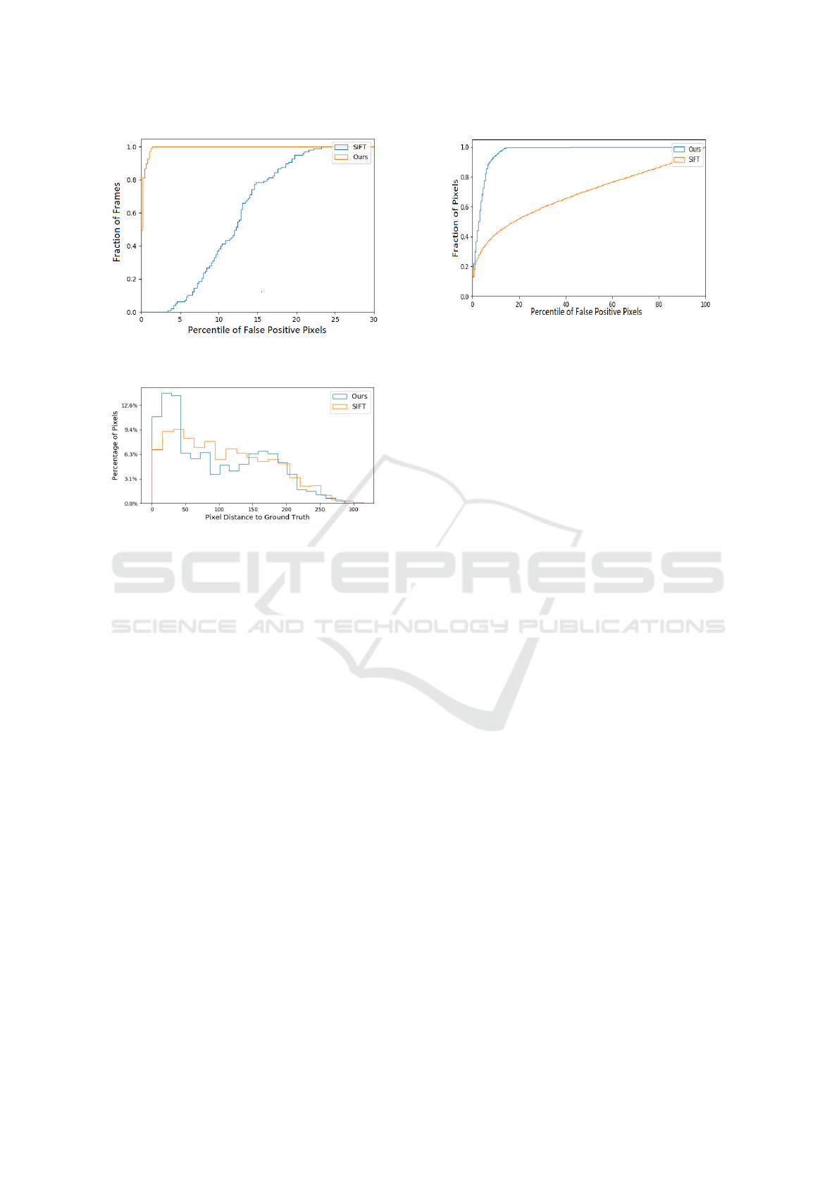
Figure 5: Cumulative histogram of false positive pixels av-
eraged over a frame between consecutive frames in a video.
Figure 6: Correspondence error histogram for keypoints se-
lected through SIFT. We show the pixel distance of the esti-
mated corresponding point to the ground truth correspon-
dence for images of size 640*480. The presented result
considers a different combination of input images based on
train and test images with same and different backgrounds.
couldn’t make the same setup for quantitative anal-
ysis. Also, their method was applicable for RGB-D
videos whereas our method as far as we know is new
and work on RGB videos and so is different and can-
not be compared. We also show visual results from
the video recorded and used for training as ground
truth is not available for the same. For test 4, we cal-
culated the significant points for both the images in
comparison and determined the significant points for
both. We determined SIFT representations for these
points and representation for the corresponding pix-
els were taken from the network output. We then
compare the accuracy of the two methods against the
ground truth information to check for accuracy.
5 EVALUATION
The result for test 1 is shown in Table 2. This demon-
strates the overall capability of tracking a pixel across
multiple frames in a video and shows how close the
representations are in that. As can be seen, our
method far outperforms the SIFT method by a large
margin when the same test is conducted for the drill
Figure 7: Pixel-wise comparison between the presented
method and SIFT. The plot shows the fraction of pixels
against percentile of false positives for each pixel, for each
of the two approaches.
object. Figure 5 shows the frame-wise comparison for
the same. As can be seen, between most frames, the
presented method performs under an error of 1 per-
centile whereas SIFT results are distributed over the
range. We also evaluated the results for the rendered
hulk object. The results show a significant difference
between drill and hulk object. Our hypothesis for this
deviation is that the hulk object has a much better tex-
ture than drill and hence SIFT performs much better.
We note that training with optimized hyperparameters
for the hulk object would likely improve the result.
Test 2 results are presented in Table 1. This test com-
pares the ability of the network to find global repre-
sentation and representation for pixels not seen be-
fore. As can be seen, even upon selecting the previ-
ously unseen images and while having different back-
grounds between the images, the presented method is
able to identify the pixels with similar accuracy prov-
ing that the pixel representation found through this
method is global. It was observed during the test that
the accuracy of prediction depended on the transfor-
mation and change in images and not on whether an
image and environment has been previously seen by
the network proving that the method determines sta-
ble features. Test 3 is performed to show the pixel-
wise performance of the presented method and the re-
sult for the same is shown in Fig. 7. This shows the
overall spread of accuracy of representation, the pix-
els that are represented well and the outliers. The er-
ror percentile for our method performs well for most
pixels. As can be seen, for over two-third of the
pixels, the error percentile is under 2 percent with
close to 15% pixels under 1 percent error and outper-
forms the compared method. This is shown in Fig. 7,
it shows the performance of our method when pit-
ted against SIFT. This shows that the representation
uniquely identifies the high contrast pixels more eas-
ily, better than SIFT. Test 4 is performed to show the
Visual Descriptor Learning from Monocular Video
449
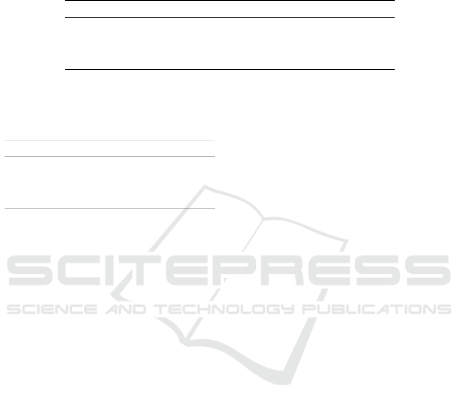
Table 1: Quantitative evaluation. We show the percentile of false correspondences in each image, averaged over the dataset.
Train refers to images where they have been exposed to the network during training. Test refers to images which are previously
unseen by the network. Train and Test notations are with respect to our network. The results are averaged over images with
same and different backgrounds selected at equal proportions.
Method Image Train-Train Train-Test Test-Test
SIFT Same Background 61.2 56.9 45.8
Our Method Same Background 3.9 8.0 3.2
SIFT Different Background 61.6 46.0 39.2
Ours Method Different Background 4.2 1.1 1.2
Table 2: Image-wise comparison of correspondence results.
Here, the error percentile for corresponding images in a
video is calculated and is averaged for the whole image and
this is repeated for subsequent 100 frame pairs in a video.
Images were sampled at 5 frames per second.
Method Object Mean Error Std Deviation
SIFT Drill 37.0 16.4
Ours Drill 0.5 0.5
SIFT Hulk 9.5 4.8
Ours Hulk 1.6 1.9
capability of the presented method for significant
points determined for SIFT algorithm, the results for
which are available in Fig. 6. We expected the SIFT
to perform well for these significant points since SIFT
was developed for this problem. But surprisingly,
even for these points, our method performed better
than SIFT in most cases as can be seen from the fig-
ure.
6 CONCLUSIONS
We introduce a method where images from a monoc-
ular camera can be used to recognize visual features
in an environment which is very important for robots.
We present an approach where optical flow calcu-
lated using a traditional method such as (Farneb
¨
ack,
2000) or using pre-trained networks as given by (Ilg
et al., 2017), (Sun et al., 2017) is used to label the
training data collected by the robot enabling it to per-
form dense correspondence of the surrounding with-
out manual intervention. For recognizing the domi-
nant object, we use a pre-trained network (Chen et al.,
2014) which is integrated into this method and can
be used without supervision. We present evidence to
the global nature of the representation generated by
the trained network where the same representation is
generated for the object present in different environ-
ments and/or at different viewpoints, transformation,
and lighting conditions. We also showed that even
in cases where a particular image and environment
is previously unseen by the network, our network is
able to generate stable features with results similar
to training images which will allow the robot to ex-
plore new environments. We quantitatively compared
our approach to a hard-engineered approach scale-
invariant feature transform (SIFT) both considering
the percentile of false positives pixels averaged over
the image and comparison at a pixel level. We show
that in both evaluations, our approach far outperforms
the existing approach. We also showed our approach’s
performance with real-world scenarios where the net-
work was trained with a video recorded using a hand-
held camera and we were able to show that the net-
work was able to generate visually stable features for
the object of interest both in previously seen and un-
seen environment thereby showing the extension of
our method to real-world scenario.
Using optical flow for labeling the positive and
negative exampled needed for contrastive loss-based
training provides us with the flexibility of replacing
the optical flow generation method with an improved
method when it becomes available and any improve-
ment in optical flow calculation will improve our re-
sults further. Similarly, for generating the mask, a
more accurate dominant object segmentation will im-
prove the presented results further. The extracted fea-
tures finds application in various fields of robotics and
computer vision such as 3D registration, grasp gen-
eration, simultaneous localization and mapping with
loop closure detection and following a human being
to a destination among others.
REFERENCES
Brachmann, E., Krull, A., Michel, F., Gumhold, S., Shot-
ton, J., and Rother, C. (2014). Learning 6D Object
Pose Estimation Using 3D Object Coordinates, vol-
ume 8690.
C. Russell, B., T. Freeman, W., A. Efros, A., Sivic, J., and
Zisserman, A. (2006). Using multiple segmentations
to discover objects and their extent in image collec-
tions. volume 2, pages 1605 – 1614.
Chen, L.-C., Papandreou, G., Kokkinos, I., Murphy, K., and
Yuille, A. L. (2014). Semantic image segmentation
VISAPP 2020 - 15th International Conference on Computer Vision Theory and Applications
450

with deep convolutional nets and fully connected crfs.
CoRR, abs/1412.7062.
Deng, J., Dong, W., Socher, R., Li, L.-J., Li, K., and Fei-
Fei, L. (2009). ImageNet: A Large-Scale Hierarchical
Image Database. In CVPR09.
Farneb
¨
ack, G. (2000). Fast and accurate motion estimation
using orientation tensors and parametric motion mod-
els. In ICPR.
Fischer, P., Dosovitskiy, A., Ilg, E., H
¨
ausser, P., Hazırbas¸,
C., Golkov, V., van der Smagt, P., Cremers, D., and
Brox, T. (2015). Flownet: Learning optical flow with
convolutional networks.
Florence, P. R., Manuelli, L., and Tedrake, R. (2018). Dense
object nets: Learning dense visual object descriptors
by and for robotic manipulation. In CoRL.
G
¨
uler, R. A., Neverova, N., and Kokkinos, I. (2018). Dense-
pose: Dense human pose estimation in the wild. 2018
IEEE/CVF Conference on Computer Vision and Pat-
tern Recognition, pages 7297–7306.
Hadsell, R., Chopra, S., and Lecun, Y. (2006). Dimen-
sionality reduction by learning an invariant mapping.
pages 1735 – 1742.
Hariharan, B., Arbelaez, P., Girshick, R., and Malik, J.
(2015). Hypercolumns for object segmentation and
fine-grained localization. pages 447–456.
He, K., Zhang, X., Ren, S., and Sun, J. (2016). Deep resid-
ual learning for image recognition supplementary ma-
terials.
Hinton, G. E., Dayan, P., Frey, B. J., and Neal, R. M. (1995).
The ”wake-sleep” algorithm for unsupervised neural
networks. Science, 268 5214:1158–61.
Ilg, E., Mayer, N., Saikia, T., Keuper, M., Dosovitskiy, A.,
and Brox, T. (2017). Flownet 2.0: Evolution of opti-
cal flow estimation with deep networks. pages 1647–
1655.
Janai, J., Guney, F., Ranjan, A., Black, M., and Geiger, A.
(2018). Unsupervised Learning of Multi-Frame Op-
tical Flow with Occlusions: 15th European Confer-
ence, Munich, Germany, September 8-14, 2018, Pro-
ceedings, Part XVI, pages 713–731.
Jia, Y., Shelhamer, E., Donahue, J., Karayev, S., Long,
J., Girshick, R. B., Guadarrama, S., and Darrell, T.
(2014). Caffe: Convolutional architecture for fast fea-
ture embedding. In ACM Multimedia.
Long, J., Shelhamer, E., and Darrell, T. (2014). Fully con-
volutional networks for semantic segmentation. Arxiv,
79.
Lowe, D. (2004). Distinctive image features from scale-
invariant keypoints. International Journal of Com-
puter Vision, 60:91–.
Reda, F., Pottorff, R., Barker, J., and Catanzaro, B. (2017).
flownet2-pytorch: Pytorch implementation of flownet
2.0: Evolution of optical flow estimation with deep
networks.
Schmidt, T., Newcombe, R. A., and Fox, D. (2017). Self-
supervised visual descriptor learning for dense corre-
spondence. IEEE Robotics and Automation Letters,
2:420–427.
Shotton, J., Glocker, B., Zach, C., Izadi, S., Criminisi, A.,
and Fitzgibbon, A. (2013). Scene coordinate regres-
sion forests for camera relocalization in rgb-d images.
pages 2930–2937.
Sivic, J., Russell, B., Efros, A., Zisserman, A., and Free-
man, W. (2005). Discovering objects and their lo-
cation in images. IEEE International Conference on
Computer Vision, pages 370–377.
Sudderth, E. B., Torralba, A., Freeman, W. T., and Willsky,
A. S. (2005). Describing visual scenes using trans-
formed dirichlet processes. In NIPS.
Sun, D., Yang, X., Liu, M.-Y., and Kautz, J. (2017). Pwc-
net: Cnns for optical flow using pyramid, warping,
and cost volume.
Taylor, J., Shotton, J., Sharp, T., and Fitzgibbon, A. (2012).
The vitruvian manifold: Inferring dense correspon-
dences for one-shot human pose estimation. vol-
ume 10.
Wang, J., song, Y., Leung, T., Rosenberg, C., Wang, J.,
Philbin, J., Chen, B., and Wu, Y. (2014). Learning
fine-grained image similarity with deep ranking. Pro-
ceedings of the IEEE Computer Society Conference on
Computer Vision and Pattern Recognition.
Wang, X. and Gupta, A. (2015). Unsupervised learning of
visual representations using videos. 2015 IEEE In-
ternational Conference on Computer Vision (ICCV),
pages 2794–2802.
Zhang, R., Lin, L., Zhang, R., Zuo, W., and Zhang, L.
(2015). Bit-scalable deep hashing with regularized
similarity learning for image retrieval and person re-
identification. IEEE Transactions on Image Process-
ing, 24:4766–4779.
Visual Descriptor Learning from Monocular Video
451
