3D Plant Growth Prediction via Image-to-Image Translation

Tomohiro Hamamoto, Hideaki Uchiyama

, Atsushi Shimada and Rin-ichiro Taniguchi

Kyushu University, Fukuoka, Japan

Keywords:

Plant Image Analysis, Prediction, CNN, LSTM, GAN, Image-to-Image Translation.

Abstract:

This paper presents a method to predict three-dimensional (3D) plant growth with RGB-D images. Based

on neural network based image translation and time-series prediction, we construct a system that gives the

predicted result of RGB-D images from several past RGB-D images. Since both RGB and depth images

are incorporated into our system, the plant growth can be represented in 3D space. In the evaluation, the

performance of our proposed network is investigated by focusing on clarifying the importance of each module

in the network. We have veriﬁed how the prediction accuracy changes depending on the internal structure of

the our network.

1 INTRODUCTION

In the ﬁeld of agricultural research, the design of plant

growth model has been conducted to manage the cul-

tivation of crops (Prasad et al., 2006). For instance,

such technologies are useful for optimizing planned

cultivation by predicting plant growth in plant facto-

ries. Plant growth prediction is obviously a challeng-

ing issue because the degree of growth varies greatly

depending on both genetic and environmental factors.

In addition, quantitative measurement of plant condi-

tions is also an important issue. To tackle the latter

issue, the conventional measurement and analysis of

the plant growth have been based on the measurement

of body weight and dry matter (Reuter and Robinson,

1997). However, such measurements are inappropri-

ate when monitoring the plant growth for a while be-

cause they need to destruct plants. Therefore, the ap-

plications of image processing has been considered as

an attempt to measure plant growth in a non-contact

manner (Mutka and Bart, 2015).

As growth indices, leaf areas, stem diameters, leaf

lengths, etc. from plants in the image are generally

used (O’Neal et al., 2002). Especially, the leaf area is

used as a basic criterion representing the plant growth.

More concretely, speciﬁc colored pixels in the images

are ﬁrst obtained via thresholding based binarization,

and then the number of pixels is used as the size of the

leaf area. Existing techniques generally focus on mea-

suring the condition of the plant growth in the images

https://orcid.org/0000-0002-6119-1184

https://orcid.org/0000-0002-2588-6894

with classical image processing methods. However,

the results do not represent physically-correct shape

in three dimensional (3D) space such that the leaf ar-

eas cannot correctly be computed in the images if the

camera is inclined against the leaves. Therefore, the

design of the plant growth model in 3D space is desir-

able for further quantitative analysis.

In this paper, we propose a method that can obtain

the 3D plant growth model from RGB-D images cap-

tured at a top view (Uchiyama et al., 2017) by using

an image-to-image translation algorithm proposed in

the ﬁeld of deep neural network. In other words, we

aim at reproducing RGB-D plant images that will be

captured several hours or several days later from past

time-series images. This issue is categorized as a fu-

ture image prediction task (Srivastava et al., 2015).

Especially, we extend the network on image-to-image

translation that changes the image domain between

images to prediction tasks. As a result, our network

outputs a future 3D plant shape by simultaneously

predicting both RGB and depth images. In the evalua-

tion, the performance of several architectures derived

from our basic one is investigated to clarify the im-

portance of each module in the network.

2 RELATED WORK

Our goal is to generate future RGB-D images based

on a time-series prediction technique so that plant

growth prediction in 3D space can be achieved. In

our approach, an image prediction technology based

Hamamoto, T., Uchiyama, H., Shimada, A. and Taniguchi, R.

3D Plant Growth Prediction via Image-to-Image Translation.

DOI: 10.5220/0008989201530161

In Proceedings of the 15th International Joint Conference on Computer Vision, Imaging and Computer Graphics Theory and Applications (VISIGRAPP 2020) - Volume 5: VISAPP, pages

153-161

ISBN: 978-989-758-402-2; ISSN: 2184-4321

153

on image-to-image translation is proposed to gener-

ate the plant growth model, as neural network based

image analysis. In this section, we discuss related

work from the following aspects: plant image anal-

ysis, image-to-image translation, and time-series pre-

dictions relevant to our study.

2.1 Plant Image Analysis

Plant image analysis has been studied since 1970s.

For instance, statistical analysis of plant growth has

been conducted simply from the size of leaves in im-

ages (MATSUI and EGUCHI, 1976). As time-series

image analysis, plant growth is analyzed by using

optical ﬂow (Barron and Liptay, 1997). In recent

years, predictive analysis based on high-quality or

large-scale plant images has been performed (Hart-

mann et al., 2011; Fujita et al., 2018).

Recently, neural networks have been used for

plant image analysis with the advance of deep learn-

ing based neural networks. Research issues such as

detection of plant leaves and measurement of plant

center positions by feature extraction tasks (Aich and

Stavness, 2017; Giuffrida et al., 2016; Chen et al.,

2017), and padding of plant image data by image gen-

eration tasks (Zhu et al., 2018) have been investigated.

In addition, there is an attempt to estimate the posi-

tion of a branch from a multi-view plant image by im-

age transformation and restore it in 3D space (Isokane

et al., 2018). One work investigated future plant im-

ages from the past images in 2D (Sakurai et al., 2019).

However, the plant growth model in 3D has not been

investigated in the literature.

2.2 Image-to-Image Translation

The basic idea of image-to-image translation is that

the source image is converted to the target image

based on learning image domain features. In the

ﬁeld of deep learning, the original image was ﬁrst

restored by auto encoder (Hinton and Salakhutdinov,

2006), and then the image synthesis by changing the

latent space is performed by using variational auto en-

coder (Kingma and Welling, 2013). VAE-GAN syn-

thesizes an image with high visual ﬁdelity by combin-

ing Generative Adversarial Network (GAN) structure

with encoder-decoder structure (Larsen et al., 2015).

In our work, we will use this idea in addition to ex-

isting time-series prediction methods for prediction

tasks.

2.3 Time-series Prediction

Time-series prediction represents the research issue to

predict future images from past ones so that what will

happen in the future is predicted. Long-Short Term

Memory (LSTM), which is a deep neural network

with a structure suitable for time series analysis, was

proposed to learn long-term relationships between

frames (Hochreiter and Schmidhuber, 1997). More

effective video representation can be achieved with

encoder-decoder structure that divides LSTM into an

encoder capturing the features of a video and a de-

coder generating a prediction image (Srivastava et al.,

2015). In addition, Convolutional LSTM, which

combines spatial convolution with LSTM structure,

has been devised to capture spatial features of im-

ages (Xingjian et al., 2015).

3 PROPOSED METHOD

Our method ﬁrst takes a series of RGB plant images

and corresponding depth images of the plants as input,

and then generates future plant images predicted from

the input through the network.

3.1 Network Architecture

We primarily use encoder-decoder LSTM to create

images to learn time-series changes of plant growth,

as similar to (Sakurai et al., 2019). Input images are

converted from time-series representation into feature

space by passing through the encoder LSTM. The de-

coder LSTM ﬁrst reads the image converted to the

feature space by the encoder, and then restores the

time-series representation from the information. It

tries to compress the amount of information by go-

ing through the transformation from image to feature

space, and allows to obtain an output image sequence

independent of the number of input images.

Further, we propose to incorporate GAN as an er-

ror function, in addition to the inter-pixel error be-

tween the output image and the correct image. We

apply GAN to the frames of the generated image se-

quence to learn the time-series characteristics. In ad-

dition, the accuracy of prediction for each image is

improved by applying GAN to one image taken at ran-

dom from the image sequence.

In summary, our network utilizes the structure of

GAN, which is divided into a generator that generates

images and a discriminator that identiﬁes images, as

illustrated in Figure 1. The generator learns so that

the generated image will be similar to the real image

VISAPP 2020 - 15th International Conference on Computer Vision Theory and Applications

154

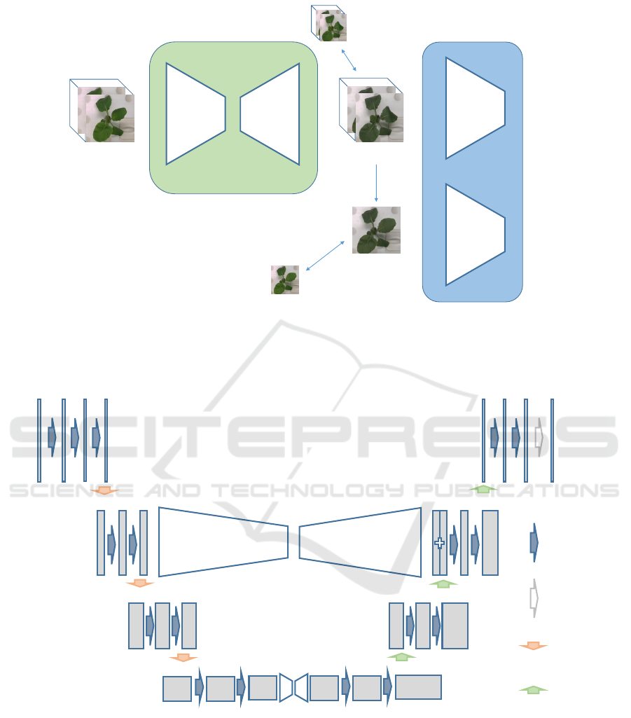
Generator

Encoder Decoder

Random

crop

real

fake

real

fake

Discriminator

Generate images

Cropped flame

MSE loss

Input images

Figure 1: Proposed network for 3D plant growth prediction. The network converts the RGB-D plant image input through the

generator into a predicted one several hours later. In the GAN process, the generated image is discriminated from the correct

image by discriminator.

2 × 2 conv

Stride = 2

Pixel shuffler

1 × 1 conv

Stride = 1

3 × 3 conv

Stride = 1

LSTM1

LSTM2

4 16 16 16 4

32 32 32 32+32 64 64

64 64 64 64

128

256

Encoder LSTM

Decoder LSTM

16 16 16

Input images Generate images

1/2 size

1/4 size

1/8 size

Figure 2: Generator. Each image is spatially convoluted through the CNN, and transformed with time information through

the LSTM. The converted image is restored by CNN and pixel shufﬂer.

while the discriminator learns to distinguish the ac-

tual image from the image synthesized by the genera-

tor. We try to reﬁne more realistic images by learning

these iteratively. In the learning process, the mean

squared error (MSE) between pixels of the images is

considered as a loss to stabilize the learning, in addi-

tion to the loss of GAN.

3.2 Generator

The generator has an encoder-decoder structure, and

uses LSTM between each of encoder and decoder, as

illustrated in Figure 2. The encoder plays the role of

dimension compression while the decoder plays the

role of restoring the image from the compressed in-

3D Plant Growth Prediction via Image-to-Image Translation

155

LSTM1 (1/2 size input) LSTM2 (1/8 size input)

Encoder LSTM

Decoder LSTM

Encoder LSTM

cell state and output

Decoder LSTM

cell state and output

mean

LSTM output

Input

Output

Figure 3: Encoder-decoder LSTM. The encoder of LSTM1 has an input that averages two elements of 1/2 size of the original

image, and LSTM2 takes 1/8 element of the original image as input. The decoder receives the output and cell state of the ﬁnal

layer of the encoder.

formation. In the encoder, the image information is

compressed by CNN, and then the time information

is compressed by encoder LSTM. In the decoder, the

number of image representations obtained as output is

generated from the time information compressed by

the encoder LSTM, and then the original image size

is restored by CNN. Regarding CNN computation,

spatial features are obtained by calculating weighted

sums with surrounding pixels in multiple layers for

each image. The image size can be compressed by

changing the kernel stride. Pixel shufﬂer is a tech-

nique to increase the size of an image by applying

array transformation to the channel, and is used for

tasks such as generating super-resolution images.

3.3 Encoder-decoder LSTM in

Generator

Images extracted by CNN are converted into output

images through two LSTM structures with different

sizes, as illustrated in Figure 3. The upper LSTM

reads local changes between images while the lower

LSTM does global changes of images. In the encoder,

the input arranged in time series is put into the LSTM

in order. The cell state and output are updated by the

spatio-temporal weight calculation with the input of

the previous time. The output at the encoder is used

only for updating the next state, and then the output at

the ﬁnal layer is passed to the decoder along with the

cell state. In the decoder, the output of the encoder is

given as the input of the ﬁrst layer, and then the in-

put of the subsequent layer is given the output of the

previous layer of the decoder itself. The decoder can

generate the output in a self-recursive manner, which

allows to generate output independent of the number

of inputs. Both encoder and decoder are implemented

by using convolutional LSTM, which is used for time-

series image analysis.

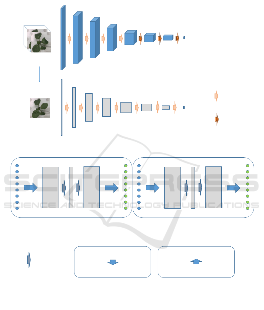
3.4 Discriminator

The discriminator performs discrimination for single

image and time-series change between images in par-

allel, as illustrated in Figure 4. The time-series dis-

criminator performs the dimensional compression of

the image in the 2D convolution part, and then iden-

tiﬁes the time series features by 3D convolution. The

single image discriminator takes out one random im-

age from the generated time-series images, and per-

forms feature extraction by two-dimensional convo-

lution.

The discriminator classiﬁes the output of the ﬁnal

layer into a binary class of 0 to 1 by activating it with

a sigmoid. When learning the generator, it learns so

that the output is 1 for the generated image with the

weight of the discriminator ﬁxed. When learning the

discriminator, the generator weight is ﬁxed so that the

correct image output is 1 and the generated image out-

put is 0. Based on this GAN property, the loss func-

tion of the generator G and the loss function of the

discriminator D are set. Since our network has two

discriminators, the loss function of a time-series dis-

criminator is denoted as G

, D

, and the loss function

of a single image discriminator is denoted as G

, D

In order to stabilize the learning process, MSE loss

VISAPP 2020 - 15th International Conference on Computer Vision Theory and Applications

156

Random

crop

Generate images

Cropped flame

16 32

64 128

128

16 32

64 128

128

[8,8,8] [4,4,4] [2,2,2]

[1,1,1]

2 × 2

2Dconv

2 × 2 × 2

3Dconv

0~1

Real or fake

0~1

Real or fake

(channel)

Figure 4: Discriminator. The discriminator has a single image identiﬁcation function and a time-series image identiﬁcation

function. 3D convolution is used for the time-series image discrimination.

Encoder_Decoder1 (1/2 size input)

Channel

concat

Channel

divide

32m

32n

m input

n output

Channel

concat

Channel

divide

128m

128n

m input

n output

128

Encoder_Decoder2 (1/8 size input)

128

3 × 3 conv

Stride = 1

Channel concat

[time, batch, height, width, channel]

[batch, height, width, time*channel]

Channel divide

[time, batch, height, width, channel]

[batch, height, width, time*channel]

Figure 5: Encoder-decoder with time-series inter-channel concatenation. The time information is compressed and decom-

pressed by combining the time axes with channels.

MSE

is added during generator learning. The loss

function of the generator L

and the loss function of

the discriminator L

in the whole network are as fol-

lows. α = 10

−3

, β = 10

−3

is given as the experimental

value.

= L

MSE

+ αG

+ βG

(1)

= αD

+ βD

(2)

As the learning activation function, relu is used for

the ﬁnal layer of the generator, sigmoid is used for the

ﬁnal layer of the classiﬁer, tanh is used for the LSTM

layer, and leaky relu is used for the other layers.

4 EVALUATION

To investigate the performance of our proposed

method, the evaluation with both RGB and depth im-

ages in the KOMATSUNA dataset (Uchiyama et al.,

2017) was performed. Especially, the effectiveness of

3D Plant Growth Prediction via Image-to-Image Translation

157

each module is investigated by removing LSTM and

GAN from our network for the comparison. In addi-

tion, we present the result of the plant growth predic-

tion in 3D.

4.1 Dataset

In our study, we used the KOMATSUNA dataset in

this evaluation. This dataset is composed of time-

series image sequences of 5 Komatuna vegetables.

For each plant, there are 60 frames taken every 4

hours from a bird’s-eye view. In this experiment,

both RGB and depth images included in the dataset

are used. This dataset assumes an environment where

data can be obtained uniformly by plant factories.

In the experiment, plant data is divided into a

training set and a test one. During the network train-

ing, four plants were used as a training set, and the

remaining one was used as a test set. The resolution

of the image is [128, 128]. For each plant, images are

reversed left and right, and rotated by 90, 180, and

270 degrees, as data augmentation.

In addition, the change of the generated image due

to the multiple layers of LSTM was veriﬁed. The ex-

periment uses a structure in which three layers of dif-

ferent LSTMs are superimposed on each of the en-

coder and decoder.

4.2 Comparison Network

To investigate the effectiveness of our network archi-

tecture, we made comparison networks by changing

our structure at the structure of the encoder-decoder

part of the network described in Section 3.

In order to investigate the change of the generated

image with and without LSTM, we used the encoder-

decoder structure based on the time series operation

by the sequence conversion between channels, which

is not based on LSTM. Dimensional compression is

performed by concatenating input images into chan-

nels and convolving them at once. In the subsequent

convolution, the amount of information in the im-

age sequence is restored by increasing the number of

channels.

Furthermore, the output of the network with and

without GAN is displayed to examine changes to

GAN. As a loss function without GAN, the network

only calculates the MSE loss for the generator.

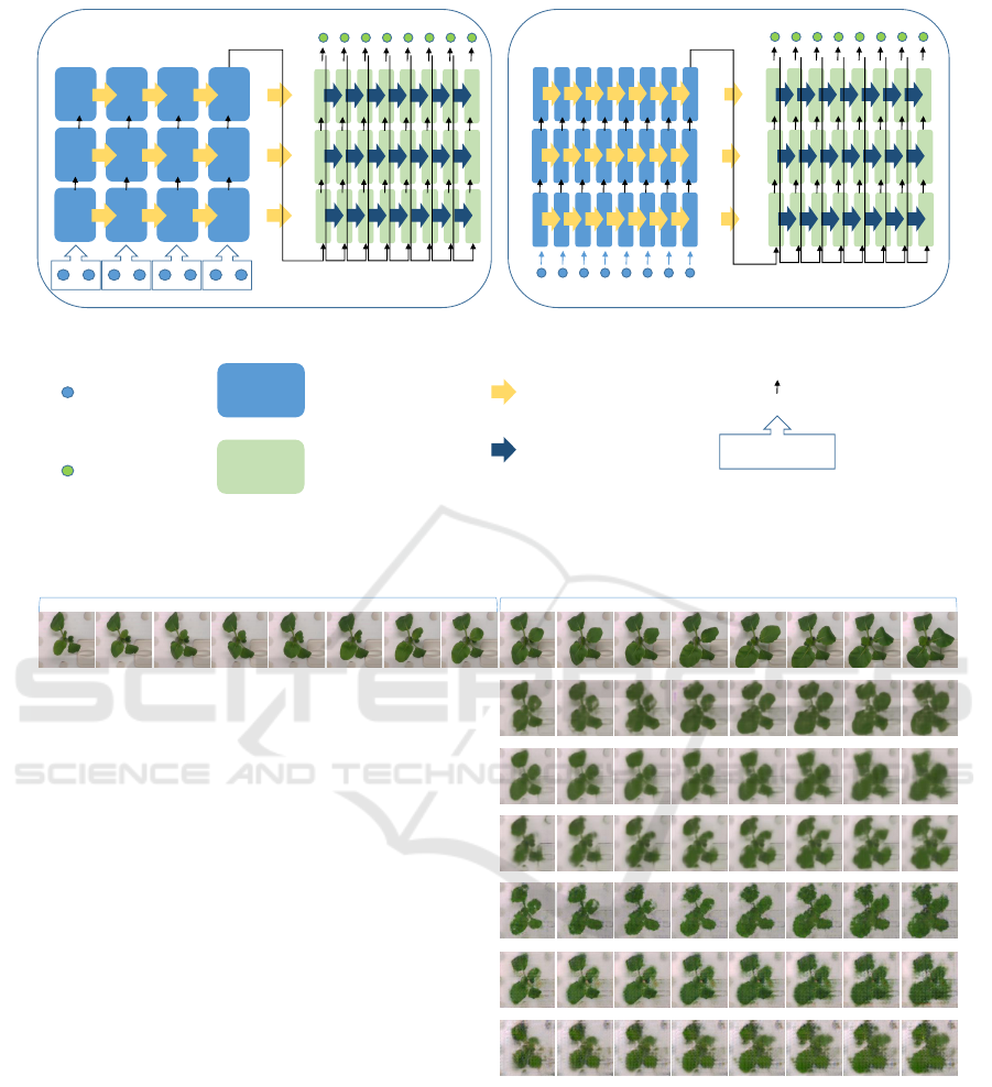
4.3 Result

The train trained an image sequence of four strains of

plants through the network, and predicted the growth

of the remaining one plant strain from the images

through the trained network. The input is a time-

series image of 8 plants. Based on the input, the future

growth of the plant is predicted and output as an im-

age. Figure 7 shows the results of learning for each

network.

Images generated by channel-concatenation

encoder-decoder are high reproducible as individual

images, and there is little blurring of the image

for the later prediction. On the other hand, the

image generated by encoder-decoder LSTM tends to

maintain the continuity of motion over time, although

the image is less sharp due to the prediction in the

back. Increasing the layer of LSTM improves the

sharpness of the image, but overreacts to movement.

As a result of applying a discriminator by GAN,

a clearer image was generated, but a real image could

not be generated. The reason is that the network be-

comes more sensitive to changes, and the response to

minute differences becomes too high.

Table 1 shows the MSE loss values calculated for

each predicted time and the average value for the im-

ages output in the network. The loss values are higher

in the later prediction, and this trend is particularly

strong when LSTM is not used. In a network with

three layers of LSTM, the MSE loss is higher than

when only one layer of LSTM is used.

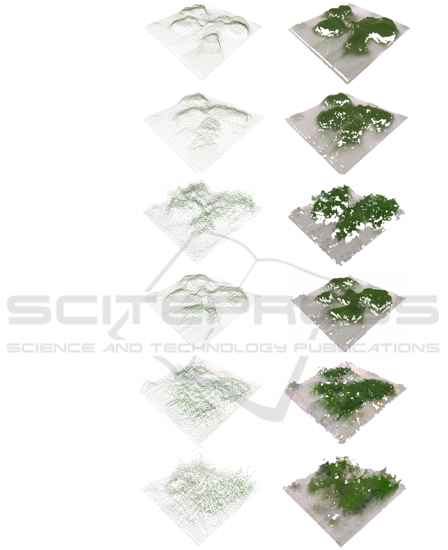
4.4 3D Reconstruction

By predicting the depth image, the prediction result

can be displayed in 3D. The depth image prediction

can be performed simultaneously with RGB predic-

tion by adding a channel for depth image prediction.

In order to generate a more natural 3D model, it is

recommended to replace missing values in the depth

image with standard values such as the median of the

image as a preliminary preparation.

The 3D model of plants predicted using RGB-D

images is displayed, as shown in Figure 8. The sur-

face of the point cloud was applied using Meshlab’s

ball pivoting.

5 CONCLUSION

We proposed a method for generating 3D plant

growth model by applying a machine learning frame-

work for plant growth prediction. We applied an im-

age sequence prediction network based on time-series

changes to plant images, and veriﬁed how the gener-

ated images change in response to changes in the net-

work structure. It was shown that 3D growth predic-

tion is performed using RGB-D images for prediction.

VISAPP 2020 - 15th International Conference on Computer Vision Theory and Applications

158

1 1 1 1

1 1 1 1 1 1 1 1

3 3 3 3 3 3 3 3

2 2 2 2 2 2 2 2

3 3 3 3 3 3 3 3

2 2 2 2 2 2 2 2

1 1 1 1 1 1 1 1

2 2 2 2

3 3 3 3

2 2 2 2 2 2 2 2

1 1 1 1 1 1 1 1

LSTM1 (1/2 size input) LSTM2 (1/8 size input)

Encoder LSTM

Decoder LSTM

Encoder LSTM

cell state and output

Decoder LSTM

cell state and output

mean

LSTM output

Input

Output

Figure 6: 3-layer encoder-decoder LSTM. The LSTM output is passed to the next LSTM. The output of the last layer of the

decoder LSTM is regarded as the output of the entire encoder-decoder.

Input images Ground truth

Channel concat

1-layer LSTM

3-layer LSTM

Channel concat +

GAN

1-layer LSTM +

GAN

3-layer LSTM +

GAN

Figure 7: Image sequence generated through network based on given input image sequence. The time-series images of 8

plants are input, (left) and the subsequent growth is output as 8 images (right).

As a future work, we will perform quantitative

analysis of the growth factors by the network by

adding to the prediction network data that is an in-

dicator of plant growth such as leaf area in addition to

the image. In addition, by inputting data such as the

amount of water given together with images, it is nec-

essary to develop a responsive system that presents

the possibility of poor growth for growing plants.

ACKNOWLEDGMENT

A part of this work is supported by JSPS KAKENHI

Grant Number JP17H01768 and JP18H04117.

3D Plant Growth Prediction via Image-to-Image Translation

159

Channel concat

1-layer LSTM

3-layer LSTM

Channel concat + GAN

1-layer LSTM + GAN

3-layer LSTM + GAN

Figure 8: 3D restoration result of predicted image. 3D point cloud (left) and faceted image by Ball Pivoting (right) are

visualized.

VISAPP 2020 - 15th International Conference on Computer Vision Theory and Applications

160

Table 1: MSE loss of the generated images: output per hour and its mean.

model leaf1 leaf2 leaf3 leaf4 leaf5 leaf6 leaf7 leaf8 mean

RGB Channel concat 0.707 1.006 1.009 1.413 1.800 1.867 2.324 2.754 1.610

+ GAN 0.975 1.364 1.371 1.636 2.060 2.348 2.587 2.949 1.911

(10

−2

) 1-layer LSTM 0.866 1.284 1.127 1.759 2.446 2.286 2.228 2.282 1.785

+ GAN 0.913 1.368 1.200 1.692 2.107 2.043 2.256 2.453 1.754

3-layer LSTM 1.629 1.454 1.463 2.182 2.745 2.679 2.912 3.029 2.262

+ GAN 1.564 1.377 1.305 2.053 2.560 2.685 2.993 3.100 2.205

Depth Channel concat 1.846 2.328 2.619 2.998 3.264 3.200 2.751 3.107 2.764

+ GAN 2.994 3.100 3.249 3.292 3.477 3.239 2.577 2.623 3.069

(10

−4

) 1-layer LSTM 1.730 1.998 2.424 2.735 3.305 3.236 2.690 2.567 2.586

+ GAN 1.916 2.072 2.457 2.719 3.344 3.359 3.142 3.408 2.802

3-layer LSTM 1.856 2.108 2.495 2.781 3.331 3.311 2.826 2.817 2.690

+ GAN 2.558 2.665 3.050 3.239 3.687 3.614 3.328 3.495 3.204

REFERENCES

Aich, S. and Stavness, I. (2017). Leaf counting with deep

convolutional and deconvolutional networks. In Pro-

ceedings of the IEEE International Conference on

Computer Vision, pages 2080–2089.

Barron, J. and Liptay, A. (1997). Measuring 3-d plant

growth using optical ﬂow. Bioimaging, 5(2):82–86.

Chen, Y., Ribera, J., Boomsma, C., and Delp, E. (2017). Lo-

cating crop plant centers from uav-based rgb imagery.

In Proceedings of the IEEE International Conference

on Computer Vision, pages 2030–2037.

Fujita, M., Tanabata, T., Urano, K., Kikuchi, S., and Shi-

nozaki, K. (2018). Ripps: a plant phenotyping system

for quantitative evaluation of growth under controlled

environmental stress conditions. Plant and Cell Phys-

iology, 59(10):2030–2038.

Giuffrida, M. V., Minervini, M., and Tsaftaris, S. A. (2016).

Learning to count leaves in rosette plants.

Hartmann, A., Czauderna, T., Hoffmann, R., Stein, N., and

Schreiber, F. (2011). Htpheno: an image analysis

pipeline for high-throughput plant phenotyping. BMC

bioinformatics, 12(1):148.

Hinton, G. E. and Salakhutdinov, R. R. (2006). Reducing

the dimensionality of data with neural networks. sci-

ence, 313(5786):504–507.

Hochreiter, S. and Schmidhuber, J. (1997). Long short-term

memory. Neural computation, 9(8):1735–1780.

Isokane, T., Okura, F., Ide, A., Matsushita, Y., and Yagi,

Y. (2018). Probabilistic plant modeling via multi-

view image-to-image translation. In Proceedings of

the IEEE Conference on Computer Vision and Pattern

Recognition, pages 2906–2915.

Kingma, D. P. and Welling, M. (2013). Auto-encoding vari-

ational bayes. arXiv preprint arXiv:1312.6114.

Larsen, A. B. L., Sønderby, S. K., Larochelle, H., and

Winther, O. (2015). Autoencoding beyond pixels

using a learned similarity metric. arXiv preprint

arXiv:1512.09300.

MATSUI, T. and EGUCHI, H. (1976). Computer control

of plant growth by image processing. Environment

Control in Biology, 14(1):1–7.

Mutka, A. M. and Bart, R. S. (2015). Image-based pheno-

typing of plant disease symptoms. Frontiers in plant

science, 5:734.

O’Neal, M. E., Landis, D. A., and Isaacs, R. (2002). An

inexpensive, accurate method for measuring leaf area

and defoliation through digital image analysis. Jour-

nal of Economic Entomology, 95(6):1190–1194.

Prasad, A. K., Chai, L., Singh, R. P., and Kafatos, M.

(2006). Crop yield estimation model for iowa using

remote sensing and surface parameters. International

Journal of Applied Earth Observation and Geoinfor-

mation, 8(1):26–33.

Reuter, D. and Robinson, J. B. (1997). Plant analysis: an

interpretation manual. CSIRO publishing.

Sakurai, S., Uchiyama, H., Shimada, A., and Taniguchi, R.-

I. (2019). Plant growth prediction using convolutional

lstm. In 14th International Conference on Computer

Vision Theory and Applications, VISAPP 2019-Part

of the 14th International Joint Conference on Com-

puter Vision, Imaging and Computer Graphics Theory

and Applications, VISIGRAPP 2019, pages 105–113.

SciTePress.

Srivastava, N., Mansimov, E., and Salakhudinov, R. (2015).

Unsupervised learning of video representations using

lstms. In International conference on machine learn-

ing, pages 843–852.

Uchiyama, H., Sakurai, S., Mishima, M., Arita, D.,

Okayasu, T., Shimada, A., and Taniguchi, R.-i.

(2017). An easy-to-setup 3d phenotyping platform

for komatsuna dataset. In Proceedings of the IEEE

International Conference on Computer Vision, pages

2038–2045.

Xingjian, S., Chen, Z., Wang, H., Yeung, D.-Y., Wong, W.-

K., and Woo, W.-c. (2015). Convolutional lstm net-

work: A machine learning approach for precipitation

nowcasting. In Advances in neural information pro-

cessing systems, pages 802–810.

Zhu, Y., Aoun, M., Krijn, M., Vanschoren, J., and Campus,

H. T. (2018). Data augmentation using conditional

generative adversarial networks for leaf counting in

arabidopsis plants. In BMVC, page 324.

3D Plant Growth Prediction via Image-to-Image Translation

161