
Model-centered Ensemble for Anomaly Detection in Time Series
Erick L. Trentini, Ticiana L. Coelho da Silva, Leopoldo Melo Junior and Jose F. de Macêdo
Insight Data Science Lab, Fortaleza, Brazil
Keywords:
Time Series, Anomaly Detection, Ensemble.
Abstract:
Time-series anomalies detection is a fast-growing area of study, due to the exponential growth of new data
produced by sensors in many different contexts as the Internet of Things (IOT). Many predictive models have
been proposed, and they provide promising results in differentiating normal and anomalous points in a time-
series. In this paper, we aim to find and combine the best models on detecting anomalous time series, so
that their different strategies or parameters can contribute to the time series analysis. We propose TSPME-AD
(stands for Time Series Prediction Model Ensemble for Anomaly Detection). TSPME-AD is a model-centered
based ensemble that trains some of the state-of-the-art predictive models with different hyper-parameters and
combines their anomaly scores with a weighted function. The efficacy of our proposal was demonstrated in
two real-world time-series datasets, power demand, and electrocardiogram.
1 INTRODUCTION
Stock market prices, sleep monitoring, trajectories of
moving objects are real-world data commonly regis-
tered taking into account some notion of time. When
collected together, the measurements compose what
is known as a time series.
Collecting vast volumes of time series data opens
up new opportunities to discover hidden patterns. As
an example, doctors can be interested in searching for
anomalies in the sleep patterns of a patient. In the mo-
bility data domain, for instance, a new interest in tra-
jectory anomaly research has occurred, which can be
integrated with navigation to provide dynamic routes
for drivers or travelers. Besides, this research can pro-
vide accurate real-time advisor routes compared with
navigation based on static traffic information. An-
other application is for taxi companies that may ob-
serve drivers with traveling trajectories that are dif-
ferent from the popular choices of other drivers and
detect fraudulent behavior.
There is a range of different approaches that ad-
dress the problem of anomaly detection on time se-
ries. Several techniques can be applied to per-
form such tasks using predictive models, clustering-
based methods, distance-based methods, among oth-
ers (Meng et al., 2018). However, detecting anoma-
lies in sequence learning tasks become challeng-
ing using standard approaches based on mathemati-
cal models that rely on stationarity (Malhotra et al.,
2016). The state-of-the-art has been investigating
LSTM neural networks (Hochreiter and Schmidhu-
ber, 1997) to overcome these limitations and to model
the normal behavior of a time series, then accurately
detect deviations from normal behaviour without any
pre-specified threshold or preprocessing phase (Mal-
hotra et al., 2015; Malhotra et al., 2016).
In this paper, we follow a similar idea. We use
some predictors, based on LSTM neural network to
model normal behavior, and subsequently, use the
prediction errors to identify anomalies. These net-
work models are data-hungry techniques and require
a massive amount of training data. We profit from the
fact that there are a plethora of instances of normal
behavior than anomalous to employ these techniques.
The intuition behind is that the network model would
only have seen instances of normal behavior during
training and the model can reconstruct them. When
given an anomalous time series, it may not be able
to rebuild it properly, and it would end up with higher
reconstruction errors than for non-anomalous time se-
ries.
We propose TSPME-AD (stands for Time Series
Prediction Model Ensemble for Anomaly Detection).
TSPME-AD combines two state-of-the-art detection
models (Malhotra et al., 2016; Malhotra et al., 2015)
to derive a combined decision. Various classifier com-
bination schemes have been devised and it has been
experimentally demonstrated that some of them con-
sistently outperform a single best classifier (Kittler
700
Trentini, E., Coelho da Silva, T., Melo Junior, L. and F. de MacÃłdo, J.
Model-centered Ensemble for Anomaly Detection in Time Series.
DOI: 10.5220/0008985507000707
In Proceedings of the 12th International Conference on Agents and Artificial Intelligence (ICAART 2020) - Volume 2, pages 700-707
ISBN: 978-989-758-395-7; ISSN: 2184-433X
Copyright
c
2022 by SCITEPRESS – Science and Technology Publications, Lda. All rights reserved

et al., 1996). In the experimental section, we prove
that by using an ensemble of such classifiers, the final
model improves in terms of F-measure on detecting
anomalous behavior.
This paper investigates a challenging problem
since the anomaly detection is performed on multi-
variate time series data. As discussed in (Wang et al.,
2018), anomalies may occur in only a subset of di-
mensions (variables). Another drawback is the loca-
tions and lengths of anomalous sub-sequences may be
different in different dimensions. Third, the anoma-
lous time series may look normal in each dimension
individually, but their combinations may be anoma-
lous.
The remainder of the paper is structured as fol-
lows: Section 2 introduces formally the problem
statement. Section 3 presents the preliminary con-
cepts to understand our approach. Section 4 presents
our proposal. Section 5 presents the related works.
Section 6 discusses the experimental evaluation, and
finally Section 7 draws the final conclusions.
2 PROBLEM STATEMENT
Consider a multivariate time series X =
[x
(1)
, x
(2)
, . . . , x
(n)
] such that x
(i)
∈ R
m
is a m-
dimensional vector x
(i)
= [x
(i)
1
, x
(i)
2
, . . . , x
(i)
m
] at
time t = i. Usually, the predictive models seek
to predict the next point given a time series.
That is, for a predictive model M and a time
series X = [x
(1)
, x
(2)
, . . . , x
(n)
], M(x
(i)
) = x
(i+1)
.
Some models may differ from this perspective,
such as predicting more than one data point,
M(x
(i)
) = [x
(i+1)
, x
(i+2)
], or re-building the time-
series backwards M(x
(i)
) = x
(i−1)
.
Given a predictive model M and a time series X,
Y = M(X ) is the predicted sequence of X using M
such that Y = [y
(1)
, y
(2)
, . . . , y
(n)
], and y
(i)
is the at-
tempt from M to build x
(i)
. Our goal is to reconstruct
the sequence X , compute the prediction errors based
on the prediction M(x
(i)
) compared to x
i
, compute
the anomaly scores (using the error distribution) and
identify the anomalies on X.
3 PRELIMINARIES
This section discusses the network architectures used
by our approach introduced in (Malhotra et al., 2015;
Malhotra et al., 2016). Our proposal is an ensemble
model that combines both strategies.
3.1 Stacked LSTM
Consider two sets of time series: s
N
for training the
prediction model M and v
N
for validating M. Let
s
N
= [s
(1)
N
, s
(2)
N
, . . . , s
(n)
N
] such that s
(i)
N
∈ R
m
is a m-
dimensional vector s
(i)
N
= [s
(i)
N
1
, s
(i)
N
2
, . . . , s
(i)
N
m
] at time
t = i. The same applies for v
N
.
For s
(i)
N
, each one of the m dimensions (s
(i)
N
∈ R
m
)
is taken by one unit in the input layer, and there is one
unit in the output layer for each of the l future predic-
tions for each of the m dimension. The LSTM units in
a hidden layer are fully connected through recurrent
connections. (Malhotra et al., 2015) stacks LSTM
layers such that each unit in a lower LSTM hidden
layer is fully connected to each unit in the LSTM
hidden layer above it through feedforward connec-
tions. Figure 1 shows the Stacked LSTM architec-
ture. The prediction model M is learned using the
non-anomalous training sequence s
N
.
Input
Layer
LSTM LSTM
Output
Layer
Figure 1: Stacked LSTM model as proposed by (Malhotra
et al., 2015).
Consider X a set of time series, and a predic-
tion length of l, each of the selected d dimensions
of x
(t)
∈ X for l < t ≤ n − l is predicted l times.
Error vectors are computed for each x
(t)
such that
e
(t)
= [e
(t)
11
, . . . , e
(t)
1l
, . . . , e
(t)
d1
, . . . , e
(t)
dl
] where e
(t)
i j
is the
difference between x
(t)
i
and the value predicted by the
model M at time t − j. In (Malhotra et al., 2015),
the prediction model trained on s
N
is used to com-
pute the error vectors for each point in the validation
and test sequences. The error vectors are modelled
to fit a multivariate Gaussian distribution N (µ, Σ) .
The validation set is used to estimate µ and Σ us-
ing Maximum Likelihood Estimation. The anomaly
score p
(t)
of an error vector e
(t)
is given by the value
of N at e
(t)
, in other words, p
(t)
is computed as
(e
(t)
− µ)
T
Σ
(−1)
(e
(t)
− µ) for an observation x
(t)
. For
x
(t)
, the value predicted is considered as anomalous if
the p
(t)
> τ, else it is classified as normal. The value
of τ is learned using v
N
by maximizing F1-score (con-
sidering a classification problem where that anoma-
lous points belong to a class and normal points to an-
other class).
3.2 Encoder Decoder Model
The network architecture discussed in this section
is composed of an LSTM-based encoder that learns
Model-centered Ensemble for Anomaly Detection in Time Series
701

fixed-length vector representation of the input time-
series. And an LSTM-based decoder that uses this
representation to reconstruct the time-series using the
current hidden state and the value predicted at the pre-
vious time-step. The network architecture was pro-
posed in (Malhotra et al., 2016) and it is illustrated in
Figure 2.
LSTM
Decoder
LSTM
Encoder
h
1
h
2
h
3
x
1
x
2
x
3
x'
1
x'
2
x'
3
h
4
x
4
h'
1
h'
2
h'
3
h'
4
Initialize with
internal state
x'
4
Input
Output
Figure 2: Encoder-Decoder model as proposed by (Malho-
tra et al., 2016).
In general, by using Encoder Decoder architec-
ture, the representation is learned from the entire
sequence which is then used to reconstruct the se-
quence. This is different from usual prediction based
anomaly detection models. Given s
N
for training the
prediction model M, h
(i)
E
is the hidden state of encoder
at time t
i
for each i ∈ {1, 2, ..., n} where h
(i)
E
∈ R
c
,
c is the number of LSTM units in the hidden layer
of the encoder. The encoder and decoder are jointly
trained to reconstruct the time series in reverse order
as {s
(n)
N
, s
(n−1)
N
, . . . , s
(1)
N
}. The final state h
(n)
E
of the
encoder is used as the initial state for the decoder.
A linear layer on top of the LSTM decoder layer is
used to predict the target. During the decoding phase,
the decoder uses s
(i)
N
and the internal state h
(i−1)
D
to
predict s‘
(i−1)
N
corresponding to target s
(i−1)
N
. Let s
N
be a set of normal training sequences, the encoder
decoder model is trained to minimize the objective
∑
s
(i)
N
∈ s
N
∑
n
i=1
s
(i)
N
− s‘
(i)
N
2
.
For an observation, x
(t)
, the anomaly score p
(t)
in
(Malhotra et al., 2016) is computed similarly as ex-
plained in the last section by modeling the error vec-
tors to fit a Multivariate Gaussian distribution. The
next section discusses our approach.
4 TSPME-AD: TIME SERIES
PREDICTION MODEL
ENSEMBLE FOR ANOMALY
DETECTION
In this paper, we combine the models (Malhotra
et al., 2015; Malhotra et al., 2016) using a model-
centered ensemble technique that attempts to com-
bine the anomaly score from both models built on the
same dataset. However, there exist some challenges
in the combination process. According to (Aggarwal,
2013), the main issues are normalization and com-
bination. The former corresponds to the problem of
different models may output anomaly scores not eas-
ily comparable. The latter is the problem of deciding
which combination function is the best (the minimum,
the maximum or the average). These are still open
questions, according to (Aggarwal, 2013), the liter-
ature on outlier ensemble analysis is very sparse so
the solutions for these mentioned issues are not com-
pletely known.
To address the first issue, a damping function is
applied to the anomaly scores, in order to prevent it
from being dominated by a few components (Aggar-
wal, 2013). Examples of a damping function could
be the square root or the logarithm. The second issue
is addressed in this paper by using a weighted aver-
age on the damped scores, that can be trained using
some sort of optimization algorithm. Figure 3 gives
an overview of the TSPME-AD pipe to construct the
model.
To construct the ensemble, we first calculate the
anomaly scores for each model in our ensemble as
in Figure 4, then we use a damping function on all
anomaly scores as in Figure 5, and aggregate each
set of scores using the weighted average function as
shown in Figure 6. In the experiments, we show
that the damped weighted average function (used
by TSPME-AD) performs better than the ensemble
model using the logarithm as a damping function.
With our new aggregated set of anomaly scores, we
try to find a threshold that maximizes some desired
score on the validation set as exemplified in Figure 7.
For a time series X , let the anomaly score a
i
∈
R and b
i
∈ R be computed from the prediction value
outputted by the models (Malhotra et al., 2015) and
(Malhotra et al., 2016), respectively. Our approach
uses the combination function shown in Equation 1 to
compute the anomaly score ∀x
i
∈ X :
A
i
=
w
(1)
× lna
i
+ w
(2)
× lnb
i
w
(1)
+ w
(2)
(1)
We say that x
i
is anomalous if
A
i
> τ
where τ is learned as one of the weights.
The weights w
(1)
, w
(2)
and τ are learned from the
validation set v
N
during the training phase, with w
1
,
w
2
∈ [0, 1] and τ ∈ R. And the goal is to maximize the
F1-score.
ICAART 2020 - 12th International Conference on Agents and Artificial Intelligence
702

Calculate anomaly
scores for each model
Use a damping function
on the anomaly scores
Aggregate all scores
using a weighted
average function
Set a threshold and
calculate some score
like F
1
Optimize weights and
thresholdto maximize
said score
Figure 3: The full pipe of TSPME-AD.
a
1
a
2
a
p
...
M
1
...
M
1
M
1
Figure 4: First, all models try to reconstruct the time series,
and we calculate the anomaly scores.
In this paper, we focus on the combination of the
models proposed by (Malhotra et al., 2015) and (Mal-
hotra et al., 2016), but the combination function can
be extended to any number of models with their re-
spective variations of hyper-parameters, and can be
generalized as in Equation 2.
A
i
=
w
(1)
× ln a
(1)
i
+ w
(2)
× ln a
(2)
i
+ · · · + w
(p)
× ln a
(p)
i
w
(1)
+ w
(2)
+ · · · + w
(p)
(2)
In Equation 2, p is the number of different mod-
els used to reconstruct the time series. From the au-
thors’ knowledge, none of the previous work that pro-
a
1
a
2
a
p
...
da
1
da
2
da
p
...
ln(x) ln(x) ln(x)
Figure 5: Applying a damping function to all anomaly
scores. e.g. the natural log function.
poses model-centered outlier ensemble models uses
this function or an LSTM based approach for outliers
detection (Aggarwal, 2013; Liu et al., 2012).
5 RELATED WORK
Anomaly detection models in time series have been
investigated by using machine learning and statistical
approaches as discussed in (Chandola et al., 2009).
Besides the aforementioned techniques, a new one
which is recently gaining momentum is deep learn-
ing and generally used to deal with non-linear mod-
els. However, only a few studies consider deep neural
networks for resolving outlier detection. (Kieu et al.,
2018) proposes an outlier detection framework to
identify an anomaly in multidimensional time-series
data. The framework incorporates several deep neu-
ral network-based autoencoders. The idea behind us-
ing autoencoders is they likely to fail to reconstruct
outliers using small feature space. Therefore, devia-
tions between the original input data and the recon-
structed data can be taken as indicators of outliers.
The paper (Malhotra et al., 2016) proposes an LSTM
encoder-decoder architecture that is trained to recon-
struct instances of normal behavior. When given an
anomalous time series, it may not be able to rebuild it
properly. Another paper that follows the same idea is
(Malhotra et al., 2015), however, the model proposed
stacks LSTM networks. Both paper (Malhotra et al.,
2015; Malhotra et al., 2016) solves the same prob-
lem than this approach, however, we gather the best
of both papers by combining them to derive a com-
bined decision.
da
1
da
2
da
p
...
A
W
1
W
2
W
p
Figure 6: Aggregating all sets of anomaly scores using a
weighted average function.
Model-centered Ensemble for Anomaly Detection in Time Series
703
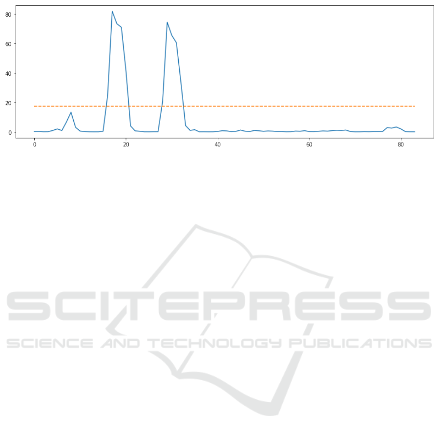
Figure 7: Setting a threshold to discriminate between ’normal’ and anomalous points.
The approach proposed in (Kong et al., 2018) can
detect long-term traffic anomaly with crowdsourced
bus trajectory data. The time series segments are ex-
tracted from bus trajectory data to describe the whole
city traffic situation from both temporal and spatial
aspects. (Kong et al., 2018) extracts the average ve-
locity and average stop time which can describe traf-
fic conditions and travel demand respectively. Then
(Kong et al., 2018) excavates poor segments which
are the bottleneck of traveling in one line by cal-
culating their anomaly index. The approach (Tariq
et al., 2019) proposes an anomaly detector for a satel-
lite system using a multivariate Convolutional LSTM
combined with a complementary Mixtures of Proba-
bilistic Principal Component Analyzer. The proposed
model learns from a large amount of normal teleme-
try data, it predicts between normal and abnormal
telemetry sequence.
Another type of anomaly detection algorithms
uses clustering techniques. Paper (Wang et al., 2018)
proposes a clustering algorithm that discretizes the
time series data into time windows, and clusters all
subsequences within each window. Univariate sub-
sequences in the same cluster within a window are
similar to each other. The behavior patterns of ob-
jects are obtained by the cluster centers, and if a time
series does not follow such behavior it is anomalous.
For multivariate time series, the algorithm transforms
the original time series into a new feature space in
which each feature is the distance to a pattern. The
smaller the distance, the more similar the data is to
the pattern. (Wang et al., 2018) performs clustering
on the transformed data, and assign anomaly score to
each time series based on the clustering results and
distances to normal cluster. Other clustered based ap-
proaches for anomaly detection are (Gao et al., 2012;
Iverson, 2004).
The main difference between TSPME-AD and
the previous one is a model-centered based approach
that uses a damped averaging function to combine
the best of the state-of-the-art detection models to
derive a combined decision. There exist few simi-
lar approaches that propose an ensemble model for
anomaly detection (Aggarwal, 2013) as (Liu et al.,
2012; Gao and Tan, 2006). However, none of these
approaches models normal behavior by profiting of
LSTM neural networks for multidimensional time se-
ries.
6 EXPERIMENTS AND RESULTS
In this section, we conduct some experiments with
two real-world datasets and report the precision, re-
call, F
1
and F
0.1
scores for TSPME-AD and the base-
line models (Malhotra et al., 2015; Malhotra et al.,
2016). We also study different combination functions
to ensemble the baseline models.
6.1 Experimental Setup
We split the dataset into 4 groups, s
n
, v
n
, v
a
, t
a
, where
s
n
and v
n
consist of a set of the time-series without
anomalies, and the other two groups (v
a
and t
a
) are
the remaining with at least one anomaly each.
We trained the models with s
n
using v
n
for early
stopping. Also, the training set (s
n
and v
n
) were used
to generate the error distribution, and then to calculate
the anomaly scores of the models.
We used the set v
a
to train the weights of the com-
bination function and the threshold τ. Finally, with
the set t
a
we calculated the anomaly scores and com-
pared TSPME-AD with the baseline models.
6.1.1 Competitors
For the stacked LSTM model, we implemented an
LSTM network with 30 and 20 LSTM nodes on the
ICAART 2020 - 12th International Conference on Agents and Artificial Intelligence
704
first and second hidden layers respectively, using the
Sigmoid activation function for the hidden layers, and
a linear activation for the output.
Since the Stacked LSTM presents as a hyper-
parameter, the number of points ahead to predict at
each step. In these experiments, we varied as 2, 4, 8
and 16 the number of points ahead to predict.
The Encoder-Decoder model only needs to re-
construct the original time-series, however there is a
hyper-parameter that is the number of hidden LSTM
units. We used the same number for the encoder and
the decoder. In the experiments, we varied the num-
ber of hidden nodes as 16, 32, 64 and 128.
6.2 Datasets
In what follows, we provide a brief overview of each
used dataset.
6.2.1 Power Demand
Figure 8: A normal week of power demand, starting at
Wednesday.
The power demand dataset provided by (Keogh
et al., 2007) registered the demand for energy sup-
ply for one year. The normal behavior is high demand
during the weekdays, and low during the weekends.
Then, the high demand on the weekends or low de-
mand on weekdays indicate for us anomalies not an-
notated.
The dataset is then sub-sampled by a factor of 8,
and broken in non-overlapping windows of 84 points,
that represent exactly one week of data. This was
also performed in (Malhotra et al., 2016). Figure 8
shows a normal behavior of power demand starting
on Wednesday.
The sets s
n
, v
n
and v
a
were built using the first
40% of dataset of the year, and the remaining to the
set t
a
. So we can better calculate the scores, as we
will have more anomalous points to test.
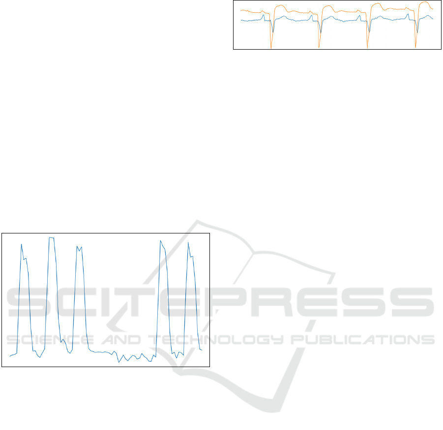
Figure 9: 4 heartbeats of the electrocardiogram dataset.
6.2.2 Electrocardiogram
The other real-world dataset is the mitdbx_108 also
provided by (Keogh et al., 2007), that depicts an elec-
trocardiogram with three distinct anomalies. This
dataset is not so well behaved like the power demand
since the heartbeat can occur at a different pace in dif-
ferent parts of the time series. This dataset is particu-
larly harder to train the encoder-decoder model since
it’s harder to find the right size and skip for the sliding
window.
This dataset is sub-sampled by a factor of 4, and
broken in non-overlapping windows of 93 points,
which represents on average one cycle of a heartbeat
of the patient’s electrocardiogram. Figure 9 shows
four cycles of a patient’s heartbeat.
As we applied in the power demand dataset, we
divided the first 40% of the e.c. to create s
n
, v
n
and v
a
and the remaining we allocated to t
a
.
6.3 Results
In this section, we present the results outputted by
TSPME-AD and its competitors. We compare our
proposal with’ Stacked LSTM (SL), and Encoder-
Decoder (ED) anomaly detection techniques. We also
evaluate the combination of these techniques using
the following ensemble strategies: Simple average
Ensemble (SA), Damped Average Ensemble (DA),
and Simple Weighted Average Ensemble (SWA).
As we mentioned before, to evaluate these
anomaly detection strategies, we use Power Demand
and Electrocardiogram datasets. We measure the per-
formance in terms of f-measure, studying two levels
of weighting between precision and recall. First, we
compute F1-score, using β = 1, which gives a bal-
anced weight to both measures. After, we compute
F
0.1
, F-measure with β = 0.1, which provides higher
weight to precision than to recall in the F-measure for-
mula. The reason to evaluate F
0.1
is the extremely
imbalanced behaviour of the time series data. As
the number of normal data is higher than the num-
ber of anomalies, an approach that produces a higher
number of false positives may not be feasible in an
anomaly detection problem. Additionally, we also an-
alyze the precision and recall separately.
Model-centered Ensemble for Anomaly Detection in Time Series
705

6.3.1 Evaluation Results from Power Demand
Dataset
Power Demand dataset is a periodic time series data.
It means that the number of points per cycle is con-
stant in time. This characteristic aids pattern recogni-
tion, and consequently, the anomaly prediction.
Table 1 shows the precision, recall, F
0.1
and F
1
for all the baseline models and the ensemble models
evaluated, trained and tested with Power Demand. As
we can see, the Simple Average (SA) and Damped
Average (DA) ensembles achieved the best results in
terms of f
0.1
and F
1
, respectively. In this experiment,
TSPME-AD achieved the second-best result in terms
of F
1
and F
0.1
.
This experiment shows that the weighted damped
average strategy of TSPME-AD achieves quality re-
sults, but it does not outperform the simple damped
average approach (DA). The great performance of
these damping strategies can be explained by the out-
put of the anomaly detection base models. A damping
average attenuates the input values before averaging.
As the output range of these models is wide, a damp-
ing strategy helps to standardize the model’s outputs.
Table 1: Test results for the Power Demand dataset.
MODELS
a
Precision Recall F
0.1
F
1
SL [K = 2] 4.42% 77.78% 0.04 0.08
SL [K = 4] 5.49% 77.78% 0.05 0.10
SL [K = 8] 22.86% 44.44% 0.22 0.30
SL [K = 16] 12.77% 66.67% 0.12 0.21
ED [H = 16] 47.06% 44.44% 0.47 0.45
ED [H = 32] 3.39% 22.22% 0.03 0.05
ED [H = 64] 59.09% 72.22% 0.59 0.65
ED [H = 128] 18.52% 27.78% 0.18 0.22
SA 100.0% 44.44% 0.98 0.61
DA 76.19% 88.89% 0.76 0.82
SWA 25.00% 72.22% 0.25 0.37
TSPME-AD 76.47% 72.22% 0.76 0.74
a
SL: Stacked LSTM, ED: Encoder Decoder, SA:
Simple Average Ensemble, DA: Damped Aver-
age ensemble, SWA: Simple Weighted Average
Ensemble, TSPME-AD: Time Series Prediction
Model Ensemble for Anomaly Detection.
6.3.2 Evaluation Results from
Electrocardiogram Dataset
As the duration of a cyclic in an electrocardiogram
varies from one instance to another, this data is called
as quasi-periodic time-series. This class of time-
series is challenging to build a prediction model be-
cause we also need to discover an average duration of
a cyclic, as done by (Malhotra et al., 2016).
As in the previous subsection, Table 2 shows the
precision, recall, F
0.1
and F
1
for all baseline models
and the ensemble model trained and tested using this
dataset. However, the TSPME-AD achieved the best
results regarding F
1
, F
0.1
, and precision, which is dif-
ferent from the results obtained using the Power De-
mand dataset. The Encoder-Decoder-based models
achieve the best recall results, but the precision score
of these models indicates that almost all normal data
are classified as anomaly data.
In this experiment, the standard ensemble fusion
strategies, such as SA, DA, and SWA, are not able to
combine the baseline models (Malhotra et al., 2015;
Malhotra et al., 2016) properly. The low performance
of these ensembles can be explained by the low per-
formance of encoder-decoder base models. The stan-
dard ensemble functions can not attenuate the poor
anomaly detection ability of Encoder-Decoder mod-
els.
We can conclude that the TSPME-AD fusion strat-
egy (using a weighted damped average function) can
compensate poor results of some anomaly detection
baseline models and produce an ensemble with better
quality results than the other fusion approaches and
baseline models individually.
It is worth to mention that TPSME-AD, in general,
outperforms the detection anomaly models from the
state-of-the-art techniques (SL and ED) as already ex-
pected since our ensemble model combines the best of
models (Malhotra et al., 2015; Malhotra et al., 2016)
on detecting anomalous time series.
Table 2: Test results for the Electrocardiogram.
MODELS
a
Precision Recall F
0.1
F
1
SL [K = 2] 22.37% 47.80% 0.22 0.30
SL [K = 4] 18.37% 57.07% 0.18 0.28
SL [K = 8] 20.97% 48.29% 0.21 0.29
SL [K = 16] 42.28% 30.73% 0.42 0.36
ED [H = 16] 7.02% 100% 0.07 0.13
ED [H = 32] 7.36% 100% 0.07 0.14
ED [H = 64] 7.37% 100% 0.07 0.14
ED [H = 128] 7.37% 100% 0.07 0.14
SA 30.84% 48.29% 0.31 0.38
DA 11.33% 60.00% 0.11 0.19
SWA 34.05% 46.34% 0.34 0.39
TSPME-AD 41.00% 47.80% 0.41 0.44
a
SL: Stacked LSTM, ED: Encoder Decoder, SA:
Simple Average Ensemble, DA: Damped Aver-
age ensemble, SWA: Simple Weighted Average
Ensemble, TSPME-AD: Time Series Prediction
Model Ensemble for Anomaly Detection.
ICAART 2020 - 12th International Conference on Agents and Artificial Intelligence
706

7 CONCLUSION AND FUTURE
WORK
In this paper, we provide an approach for anomaly
detection which combines two state-of-the-art detec-
tion models, one based on stacked LSTM and another
one encoder-decoder based. TPSME-AD, in general,
outperforms the detection anomaly models from the
state-of-the-art techniques as already expected since
our ensemble model combines the best of models
(Malhotra et al., 2015; Malhotra et al., 2016) on de-
tecting anomalous time series. In the experiments, we
also show that, for a quasi-periodic time series data,
our model can outperform also standard ensemble fu-
sion approaches, such as simple average, damped av-
erage, and simple weighted average.
As a future direction, we aim at evaluating our
proposal with other datasets like the electrocardio-
gram, and the space-shuttle valve time-series (Keogh
et al., 2007). Another future improvement can be
added to a regularization of the combination function
so that we can mitigate the overfitting in the validation
dataset.
ACKNOWLEDGMENTS
This work is partially supported by the FUNCAP SPU
8789771/2017, and the UFC-FASTEF 31/2019.
REFERENCES
Aggarwal, C. C. (2013). Outlier ensembles: position paper.
ACM SIGKDD Explorations Newsletter, 14(2):49–58.
Chandola, V., Banerjee, A., and Kumar, V. (2009).
Anomaly detection: A survey. ACM computing sur-
veys (CSUR), 41(3):15.
Gao, J. and Tan, P.-N. (2006). Converting output scores
from outlier detection algorithms into probability es-
timates. In Sixth International Conference on Data
Mining (ICDM’06), pages 212–221. IEEE.
Gao, Y., Yang, T., Xu, M., and Xing, N. (2012). An un-
supervised anomaly detection approach for spacecraft
based on normal behavior clustering. In 2012 Fifth
International Conference on Intelligent Computation
Technology and Automation, pages 478–481. IEEE.
Hochreiter, S. and Schmidhuber, J. (1997). Long short-term
memory. Neural computation, 9(8):1735–1780.
Iverson, D. L. (2004). Inductive system health monitoring.
Keogh, E., Lin, J., Lee, S.-H., and Van Herle, H. (2007).
Finding the most unusual time series subsequence: al-
gorithms and applications. Knowledge and Informa-
tion Systems, 11(1):1–27.
Kieu, T., Yang, B., and Jensen, C. S. (2018). Outlier detec-
tion for multidimensional time series using deep neu-
ral networks. In 2018 19th IEEE International Con-
ference on Mobile Data Management (MDM), pages
125–134. IEEE.
Kittler, J., Hater, M., and Duin, R. P. (1996). Combining
classifiers. In Proceedings of 13th international con-
ference on pattern recognition, volume 2, pages 897–
901. IEEE.
Kong, X., Song, X., Xia, F., Guo, H., Wang, J., and Tolba,
A. (2018). Lotad: Long-term traffic anomaly detec-
tion based on crowdsourced bus trajectory data. World
Wide Web, 21(3):825–847.
Liu, F. T., Ting, K. M., and Zhou, Z.-H. (2012). Isolation-
based anomaly detection. ACM Transactions on
Knowledge Discovery from Data (TKDD), 6(1):3.
Malhotra, P., Ramakrishnan, A., Anand, G., Vig, L., Agar-
wal, P., and Shroff, G. (2016). Lstm-based encoder-
decoder for multi-sensor anomaly detection. arXiv
preprint arXiv:1607.00148.
Malhotra, P., Vig, L., Shroff, G., and Agarwal, P. (2015).
Long short term memory networks for anomaly detec-
tion in time series. In Proceedings, page 89. Presses
universitaires de Louvain.
Meng, F., Yuan, G., Lv, S., Wang, Z., and Xia, S. (2018).
An overview on trajectory outlier detection. Artificial
Intelligence Review.
Tariq, S., Lee, S., Shin, Y., Lee, M. S., Jung, O., Chung,
D., and Woo, S. S. (2019). Detecting anomalies in
space using multivariate convolutional lstm with mix-
tures of probabilistic pca. In Proceedings of the 25th
ACM SIGKDD International Conference on Knowl-
edge Discovery & Data Mining, pages 2123–2133.
ACM.
Wang, X., Lin, J., Patel, N., and Braun, M. (2018). Exact
variable-length anomaly detection algorithm for uni-
variate and multivariate time series. Data Mining and
Knowledge Discovery, 32(6):1806–1844.
Model-centered Ensemble for Anomaly Detection in Time Series
707
