Fast Fourier Transform based Force Histogram Computation for 3D

Raster Data

Jaspinder Kaur, Tyler Laforet and Pascal Matsakis

Department of Computer Science, University of Guelph, Guelph, Canada

Keywords:

Relative Position Descriptor, Computer Vision, Image Processing, Force Histogram.

Abstract:

The force histogram is a quantitative representation of the relative position between two objects. Two practical

algorithms have been previously introduced to compute the force histogram between objects: the line-based

algorithm (which works well with 2D data, but is computationally unstable in the case of 3D data), and the

Fast Fourier Transform (FFT)-based algorithm (which is inefﬁcient in the case of 2D data, but has not been

implemented for 3D data). In this paper, an efﬁcient FFT-based algorithm for force histogram computation

in the case of 3D raster data is introduced. Its computation time is compared against that of the 3D line-

based algorithm; except in a few cases, the computation time for new FFT-based algorithm is less than that of

3D line-based algorithm. The experiments validate that the FFT-based algorithm is computationally efﬁcient

regardless of the number of directions, type of forces, and shape of the objects (convex, concave, disjoint or

overlapping).

1 INTRODUCTION

Humans often rely on the relative positioning of the

objects around them in order to understand and ex-

press spatial information. In our daily lives, the

relative position of objects is often communicated

through linguistic expressions like, “the shopping

mall is south of the apartment”, “the school is near

my home”, and “the folder is inside the case”. Spa-

tial prepositions like “north”, “inside” and “nearby”

represent spatial relationships. Distance relationships

(Ryoo and Aggarwal, 2009) describe how far apart the

objects are in space, like “far away”, “nearby”, “at”.

Directional relationships (also called cardinal or pro-

jective (Gapp, 1995) relationships) are mostly iden-

tiﬁed by words like “west”, “to the right of”. Topo-

logical relationships specify concepts of connectivity,

adjacency and enclosure (Egenhofer, 1989; Schneider

and Behr, 2005; Egenhofer, 1990).

Comprehending the spatial relationships in a

scene plays a vital role in several areas such as pat-

tern recognition, human-robot communication, scene

description in natural language, image understanding

and so forth. Models of spatial relationships (dis-

tance, directional and topological) among spatial enti-

ties are either quantitative or qualitative. In qualitative

models (Frank, 1996), a relationship either holds or

does not hold. On the other hand, in quantitative mod-

els, a relationship may hold to some degree (Deselaers

et al., 2004). Over the years, qualitative models have

been used in various areas of computer vision. How-

ever, most practical applications of computer vision

and image processing (Smeulders et al., 2000; Skubic

et al., 2001; Skubic et al., 2002; Miller and Wentz,

2003) require quantitative models called relative po-

sition descriptors (RPD).

Relative position descriptors are vectors of val-

ues that encode information about an object’s position

relative to another object. RPDs bridge the gap be-

tween low-level spatial features (e.g., pixels in an im-

age) and high level concepts (i.e spatial relationships).

An ideal relative position descriptor encapsulates all

possible spatial relationship information between ob-

jects, and allows that information to be extracted efﬁ-

ciently. Over the years, much attention has been paid

towards identifying effective approaches for mod-

elling objects’ relative positions. Several RPDs have

been introduced (Miyajima and Ralescu, 1994; Kr-

ishnapuram et al., 1993; Naeem and Matsakis, 2015).

The force histogram (Matsakis, 1998; Matsakis and

Wendling, 1999) may be one of the most well known

relative position descriptors with various theoretical

and practical applications. It encapsulates the struc-

tural information (e.g., size, shape, etc.) as well as

the spatial relationship information between objects.

So far, many algorithms for force histogram compu-

Kaur, J., Laforet, T. and Matsakis, P.

Fast Fourier Transform based Force Histogram Computation for 3D Raster Data.

DOI: 10.5220/0008985100690074

In Proceedings of the 9th International Conference on Pattern Recognition Applications and Methods (ICPRAM 2020), pages 69-74

ISBN: 978-989-758-397-1; ISSN: 2184-4313

tation have been introduced. The two main algorithms

for force histogram computation are the line-based al-

gorithm and the Fast Fourier Transform (FFT)-based

algorithm. The line-based algorithm for force his-

togram computation exists for 2D raster objects, 2D

vector objects, 3D raster objects and 3D vector ob-

jects, although the algorithms for the 3D objects are

computationally costly. On the other hand, the FFT-

based algorithm exists only for 2D raster data, and has

not yet been implemented for 3D raster objects.

This paper presents an extension of the FFT-based

algorithm for the computation of force histogram in

the case of 3D raster objects. In Section 2, we dis-

cuss the force histogram and provide a brief overview

of various algorithms found in the literature for com-

puting the force histogram. In Section 3, the algo-

rithm which involves handling 3D raster objects is

presented. Section 4 presents the experiments and a

comparative study in which the line-based force his-

togram is compared against the FFT-based force his-

togram. Section 5 concludes the discussion and pos-

tulates future work.

2 BACKGROUND

2.1 Force Histogram

A histogram of forces F

(θ) is a function from IR

(the set of directions) to IR

(the set of real numbers)

that represent the position of object A relative to ob-

ject B (Figure 1b). For a given direction θ, the value

(θ) is the sum of the magnitude of all elemen-

tary forces exerted by the points of B on those of A;

this in turn tends to move A in the direction θ (Fig-

ure 1a). Here, the object A is called the argument and

the object B is called the referent. The magnitude of

each elementary force is given by 1/|r|

, where r is

the distance between points and t is any real number.

The function F

(θ) has two special cases: t = 2, and

t = 0. When t = 2, F

(θ) is called the gravitational

force histogram, and the forces between the points are

inversely proportional to the the square of distance be-

tween them (1/r

). When t = 0, F

(θ) is called the

constant force histogram, and the forces do not de-

pend on this distance.

2.2 Algorithms for the Force Histogram

Computation

2.2.1 Line-based Algorithm

Matsakis indicates in (Matsakis, 1998; Matsakis and

Wendling, 1999) that the force histogram between ob-

Figure 1: Force histogram: (a) Consider two objects A and

B; F

(θ) is the scalar resultant of elementary forces in the

direction θ. (b) The histogram F

between the objects A

and B.

jects in an image can be computed by ﬁrst partition-

ing the image into a number of raster lines, and then

batch-processing pixels on each line. Consider ob-

jects A and B; for any oriented line Λ, F

(θ) is the

scalar resultant of elementary forces exerted by points

of B ∩Λ on those of A ∩Λ in a direction θ. In an

ideal case, the shapes of objects A and B are simple

(e.g., convex). For any direction θ, the line Λ inter-

sects each object exactly once, thus the number of

segments A ∩Λ and B∩Λ included in a line is at most

2. The computation of the force histogram is equiva-

lent to computing forces between two segments, thus

lowering the computation time. In the worst case, ob-

jects A and B have complex shapes (e.g., a fractal-like

structure or objects with multiple disconnected com-

ponents). For any direction θ, the line Λ intersects

each objects multiple times, thus the number of seg-

ments A ∩Λ and B ∩Λ may be very high. This will

lead to computing forces between multiple segments,

thus increasing the computation time.

In (Ni et al., 2004), the line-based algorithm for

force histogram computation is extended for 3D data.

The basic principal remains unchanged. For any di-

rection

θ (here deﬁned by a unit vector), the function

(

θ) is the scalar resultant of elementary forces ex-

erted by the voxels of B on those of A. The

θ is taken

from a set D

of evenly distributed reference direc-

tions (Bourke, 2007). The K reference directions in

the set D

should follow three primary constraints:

1. They should be evenly distributed in 3D space,

2. They should include six primitive directions i.e.,

(±1,0,0) (left/right), (0,±1,0) (above/below), and

(0,0,±1) (front/behind), and,

3. If a direction θ belongs to the set, then the op-

posite direction −θ should also be a part of the

direction set.

The above constraints indicate m = 6 + 8l, where

6 denotes six primitive directions, 8 denotes the re-

ICPRAM 2020 - 9th International Conference on Pattern Recognition Applications and Methods

gions demarcated by the XY, YZ, ZX plane, and l

implies the number of reference directions in each

plane. 3D data, however, is signiﬁcantly larger than

2D data, so it is necessary to follow appropriate op-

timization techniques. Therefore, a number of irrele-

vant directions are identiﬁed and dropped in order to

ease the computational burden. Forces in the remain-

ing directions are computed in a similar fashion to the

2D case. A simple yet powerful test is conducted to

drop irrelevant directions. According to the test in (Ni

et al., 2004), a direction

θ is considered relevant, if

(

θ) 6= 0 i.e., for any oriented line Λ, A∩Λ6= 0 and

B ∩Λ 6= 0. Otherwise, a direction

θ is irrelevant, and

should not be considered while computing the force

histogram F

(θ).

2.2.2 FFT-based Algorithm

The line-based algorithm that is based on the image

partitioning and batch processing of pixels (Section

2.2.1) has two signiﬁcant drawbacks: (1) the compu-

tation time is directly proportional to the number of

directions (K) in which the forces are evaluated, and

(2) it depends on the shape of the object (concave

or convex) and their relative position (overlapping

or disjoint). To solve the issues encountered by

the line-based algorithm, Matsakis and Jing Bo Ni

(Ni and Matsakis, 2010) introduced an alternative

deﬁnition for force histogram computation. Consider

A and B are the membership functions of objects in

a digital image. The image is extended through zero

padding to occupy the inﬁnite space Z

, where Z

denotes the set of all integers. .The force histogram is

derived from the mapping Ψ

deﬁned over discrete

space. The mapping Ψ

from Z

to IR is deﬁned as

follows:

(d,e) =

+∞

−∞

+∞

−∞

A(x,y)B(x + d,y + e)dx dy

(1)

This is a spatial correlation that provides raw infor-

mation about the relative positions of objects, and

can be computed quickly by using the Fast Fourier

transform (FFT). The force histogram

(θ) can

be computed using the mapping deﬁned in Equation

(1). For two objects A and B, the function

(θ) is

deﬁned by:

(θ) =

∞

θ)

dr (2)

The FFT-based algorithm has been implemented only

for 2D raster objects; it has not been implemented for

3D raster objects.

3 FFT-BASED ALGORITHM FOR

3D RASTER DATA

In this section, we introduce the ﬁrst FFT-based algo-

rithm for the computation of force histogram in the

case of 3D raster objects. The basic principle re-

mains the same. A force histogram is computed us-

ing a mapping Ψ

deﬁned over the 3D space, where

is the spatial correlation between two 3D objects.

A Fast Fourier Transform (FFT) technique is used to

compute the mapping Ψ

quickly. Section 3.1 fo-

cuses on the implementation of the spatial correlation

(Ψ

), then Section 3.2 discusses the computation of

the force histogram using Ψ

3.1 Implementation of Ψ

Consider A and B as two 3D raster objects in a

domain G

h×k×l

. Ψ

provides raw information about

the position of object A relative to object B. The

spatial correlation Ψ

between 3D raster objects A

and B is deﬁned as follows:

(d,e, f ) =

h−1

∑

h=0

k−1

∑

k=0

l−1

∑

l=0

A(x,y,z)B(x+d,y+e,z+ f )

(3)

The set G

h×k×l

= {−h + 1........h − 1}×{−k +

1........k − 1}×{−l + 1........l − 1} is the effective

domain of Ψ

. In Equation (3), we suppose

that B(x + d,y + e,z + f ) = 0, if the voxel (x + d,

y + e, z + f ) lies outside of G

h×k×l

; such that

(x + d,y + e,z + f ) /∈ {0 .. . h −1} × {0 ... k −1} ×

{0.. .l −1}. It is not difﬁcult to see that only voxels

(d,e,f) that are in the effective domain G

h×k×l

, will

satisfy Ψ

6= 0. Consider the reﬂection of object A

about the origin, such that A

(−x,−y,−z) = A(x,y,z).

By replacing A(x,y,z) with A

) in Equation 3,

where x

= −x, y

= −y and z

= −z, we get,

(d,e, f ) =

h−1

∑

h=0

k−1

∑

k=0

l−1

∑

l=0

A(x

)B(d −x, e −y, f −z)

(4)

Equation (4) refers to the 3-D discrete convolution.

Using matrix notation, we get:

[Ψ

] = [A

] ⊗[B

], (5)

where ⊗ is the convolution operator. According to

the Convolution theorem, the Fourier transform has

the power to convert the convolution operation into

an ordinary multiplication, and vice versa. Using the

Convolution theorem, equation (5) can be written as:

Fast Fourier Transform based Force Histogram Computation for 3D Raster Data

[Ψ

] = W

−1

2h−1

·W

−1

2k−1

[(W

2h−1

·W

2k−1

·[A

] ·W

2l−1

)

×(W

2h−1

·W

2k−1

·[B

] ·W

2l−1

)] ·W

−1

2l−1

(6)

where W

and W

−1

are the Fourier and inverse Fourier

transform matrices of order i and × is the matrix prod-

uct. From Equation (6), computation of [Ψ

] re-

quires three 3-D discrete Fourier transforms. Using

the Convolution theorem, Ψ

can be computed in

O(NlogN) time as this is the complexity of the Fast

Fourier transform (FFT).

3.2 Implementation of

In this section,

is computed using the spatial

correlation Ψ

(Section 3.1). Only a ﬁnite number

of directions θ are considered. A reasonable choice

for θ (Section 2.2.1) is to choose from a set of

evenly distributed reference directions D

. For 3-

dimensional objects, Equation (2) takes the following

form:

(θ) =

∞

(dcosθ,dsinθ,z)

dr (7)

The FFT-based algorithm described in this paper

runs in O(NlogN) time. The computation time for

the FFT-based algorithm is independent of the type of

forces (t) and number of directions (K) in which the

forces are measured. All objects regardless of their

shape (complex or simple) and relative position (dis-

joint or overlapping) are treated in the same manner.

The experiments conducted in Section 4 validate this.

4 EXPERIMENTS

In this section, F

denotes a force histogram com-

puted using the line-based algorithm and

denotes

a force histogram computed using the new FFT-based

algorithm. The experiments are conducted on a va-

riety of 3D raster objects. The test data consists of

objects generated from quadratic Koch island fractals

at iterations 2 and 3, overlapping objects, cubes and

segmented cubes (Figure 2). The size of the objects is

kept constant (N = 512

) for all experiments, except

for the scenario where the effect of size is investigated

on the computational time of

and F

. The al-

gorithms are implemented in C, and the experiments

were conducted on a mac OS equipped with an 2GHz

Intel Core i5 CPU and 8GB of memory. The compu-

tation time is measured using the C library function

clock().

Table 1: Tversky Index (µ

), N = 512

, K=1800.

Figure 2 (a) (b) (d)

t= 0 0.91 0.86 0.956

t= 1 0.90 0.82 0.950

t = 2 0.87 0.8 0.943

4.1 Comparing Histogram Values

This experiment demonstrates that F

and

are almost identical, as expected. The histogram

associated with the F

is denoted as h

(θ) and

the histogram associated with

is denoted as

(θ). The dissimilarity between h

(θ) and h

(θ) is

measured using the Tversky index (µ

) =

∑

K−1

i=0

min

{

(θ

),h

(θ

)

}

∑

K−1

i=0

max

{

(θ

),h

(θ

)

}

(8)

is 1 when the h

(θ) and h

(θ) histograms are ex-

actly the same and µ

is 0 when the h

(θ) and h

(θ)

histograms are orthogonal. The µ

values tend to be

close to 1 for the object pairs considered in our ex-

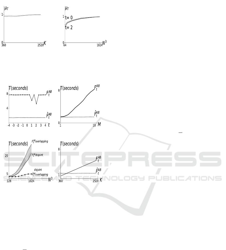
periments (Table 1). The effect of K and N on µ

has

also been studied (Figure 3). The values of µ

are al-

most independent of K (Figure 3a) but grow notably

and tend towards 1 when N increases (Figure 3b).

4.2 Comparing Computation Time

The results presented in Figure 4a shows that the com-

putation of

is independent of the choice of t;

however, F

computes faster when t=1 or t=2. The

prominent reason for this is because the computation

of each F

devolves into evaluating a number of nu-

merical expressions which are computationally faster

when t=1 and t=2.

(a) $$$$$$$$$$$$$$$$$$$$$$$$$$$$$$$$$$$$$$$$$$$$$$$(b)$$$$$$$$$$$$$$$$$$$$$$$$$$$$$$$$$$$$$$$$$$$$$$$$(c)$

!!!!!(d)!!!!!!!!!!!!!!!!!!!!!!!!!!!!!!!!!!!!!!!!!!!!!!!!(e)!

!!A!

!!B!

Figure 2: Test Data: The 3D objects used in this experiment

are right cylinders whose bases are quadratic Koch island

fractals at (a) iteration 2 and (b) iteration 3. Also shown are

ICPRAM 2020 - 9th International Conference on Pattern Recognition Applications and Methods

(a) (b)

Figure 3: (a) µ

against the number of directions (K), ob-

jects are from Figure 2b and N = 512

.(b) µ

against the

number of voxels (N), objects are from Figure 2b and K =

1800.

(a) (b)

Figure 4: In (a), the objects are from Figure 2a, K= 1800,

N = 512

. In (b), the objects are from Figure 2e, M denotes

the number of disconnected components in an object, K=

1800, N = 512

. In (c), the objects are from Figure 2(b,c),

K= 1800. In (d), the objects are from Figure 2c, N = 512

In an ideal case, the computational complexity of

is O(KN) for simple object shapes, whereas for

complex shapes (e.g, objects with multiple discon-

nected parts) the computational complexity of F

is O (KN

√

N). The main reason for this is that for

simple convex objects (Figure 2d), any line that runs

through both objects intersects each object only once;

therefore, computing a force histogram value comes

down to computing the forces between two segments.

However, for complex shapes (Figure 2e), any line

passing through both objects intersects them in multi-

ple segments; therefore, computing a histogram value

comes down to computing the forces between a large

number of segments which further leads to longer

processing times (Section 2.2.1). However, the

always computes in O(NlogN) regardless of the ob-

ject’s shape. This is illustrated by Figure 4b. Further-

more, the relative position (disjoint or overlapping) of

the objects also affects the processing time of F

whereas

stays the same for disjoint as well as

overlapping objects (Figure 4c). Finally, when K in-

creases, the processing time of F

also grows lin-

early. On the other hand,

remains constant (Fig-

ure 4d).

5 CONCLUSION

The FFT-based algorithm for the computation of force

histogram is a powerful tool to quantitatively repre-

sent the relative position between two objects. In ear-

lier work, only 2D objects were considered. In this

paper, we have shown that 3D objects can also be

handled, and efﬁciently. The FFT-based algorithm for

the force histogram computation described in this pa-

per is computed in O(NlogN) time, where N is the

number of voxels in an object. In comparison, the

line-based algorithm for the force histogram compu-

tation is computed in O (KN

√

N) time, where K is the

number of direction in which forces are computed.

Furthermore, contrary to the line-based algorithm, the

computation time of the FFT-based algorithm is inde-

pendent of the number of directions, type of forces,

shape and relative position of the objects. The FFT-

based algorithm is, therefore, an appropriate choice

over the line-based algorithm for 3D raster objects,

except for the case when the objects’ shapes are sim-

ple or when the number of directions in which the

forces are computed is small. In future work, the

φ-descriptor algorithm can also be extended for 3D

raster objects, and then the processing times and per-

formance of the force histogram and the φ-descriptor

for 3D raster objects can also be comparatively com-

pared.

REFERENCES

Bourke, P. (2007). Distributing points on a sphere.

Deselaers, T., Keysers, D., and Ney, H. (2004). Fea-

tures for image retrieval: A quantitative comparison.

In Joint Pattern Recognition Symposium, pages 228–

236. Springer.

Egenhofer, M. (1990). A mathematical framework for

the deﬁnition of topological relations. In Proc. the

fourth international symposium on spatial data hand-

ing, pages 803–813.

Egenhofer, M. J. (1989). A formal deﬁnition of binary

topological relationships. In International conference

on foundations of data organization and algorithms,

pages 457–472. Springer.

Fast Fourier Transform based Force Histogram Computation for 3D Raster Data

Frank, A. U. (1996). Qualitative spatial reasoning: Cardi-

nal directions as an example. International Journal of

Geographical Information Science, 10(3):269–290.

Gapp, K.-P. (1995). Angle, distance, shape, and their rela-

tionship to projective relations. In Proceedings of the

17th annual conference of the cognitive science soci-

ety, pages 112–117.

Krishnapuram, R., Keller, J. M., and Ma, Y. (1993). Quan-

titative analysis of properties and spatial relations of

fuzzy image regions. IEEE Transactions on fuzzy sys-

tems, 1(3):222–233.

Matsakis, P. (1998). Relations spatiales structurelles et in-

terpretation d’images. PhD thesis.

Matsakis, P. and Wendling, L. (1999). A new way to repre-

sent the relative position between areal objects. IEEE

Transactions on pattern analysis and machine intelli-

gence, 21(7):634–643.

Miller, H. J. and Wentz, E. A. (2003). Representation and

spatial analysis in geographic information systems.

Annals of the Association of American Geographers,

93(3):574–594.

Miyajima, K. and Ralescu, A. (1994). Spatial organization

in 2d segmented images: representation and recogni-

tion of primitive spatial relations. Fuzzy Sets and Sys-

tems, 65(2-3):225–236.

Naeem, M. and Matsakis, P. (2015). Relative position

descriptors. In Proceedings of the International

Conference on Pattern Recognition Applications and

Methods-Volume 1, pages 286–295. SCITEPRESS-

Science and Technology Publications, Lda.

Ni, J. and Matsakis, P. (2010). An equivalent deﬁnition of

the histogram of forces: Theoretical and algorithmic

implications. Pattern Recognition, 43(4):1607–1617.

Ni, J., Matsakis, P., and Wawrzyniak, L. (2004). Quanti-

tative representation of the relative position between

3d objects. In VIIP 2004 (4th IASTED Int. Conf. on

Visualization, Imaging, and Image Processing), pages

452–289.

Ryoo, M. S. and Aggarwal, J. K. (2009). Spatio-temporal

relationship match: video structure comparison for

recognition of complex human activities. In ICCV,

volume 1, page 2. Citeseer.

Schneider, M. and Behr, T. (2005). Topological relation-

ships between complex lines and complex regions.

In International Conference on Conceptual Modeling,

pages 483–496. Springer.

Skubic, M., Blisard, S., Carle, A., and Matsakis, P. (2002).

Hand-drawn maps for robot navigation. In AAAI

Spring Symposium, Sketch Understanding Session,

page 23.

Skubic, M., Matsakis, P., Forrester, B., and Chronis, G.

(2001). Extracting navigation states from a hand-

drawn map. In Proceedings 2001 ICRA. IEEE In-

ternational Conference on Robotics and Automation

(Cat. No. 01CH37164), volume 1, pages 259–264.

IEEE.

Smeulders, A. W., Worring, M., Santini, S., Gupta, A., and

Jain, R. (2000). Content-based image retrieval at the

end of the early years. IEEE Transactions on Pattern

Analysis & Machine Intelligence, (12):1349–1380.

ICPRAM 2020 - 9th International Conference on Pattern Recognition Applications and Methods