
Computation of the φ-Descriptor in the Case of 2D Vector Objects
Jason Kemp, Tyler Laforet and Pascal Matsakis
School of Computer Science, University of Guelph, Stone Rd E, Guelph, Canada
Keywords:
Image Descriptors, Relative Position Descriptors, φ-Descriptor, Spatial Relationships, Vector Data.
Abstract:
The spatial relations between objects, a part of everyday speech, are capable of being described within an
image via a Relative Position Descriptor (RPD). The φ-descriptor, a recently introduced RPD, encapsulates
more spatial information than other popular descriptors. However, only algorithms for determining the φ-
descriptor of raster objects exist currently. In this paper, the first algorithm for the computation of the φ-
descriptor in the case of 2D vector objects is introduced. The approach used is based on the concept of Points
of Interest (which are points on the boundaries of the objects where elementary spatial relations change)
and dividing the objects into regions according to their corresponding relationships. The capabilities of the
algorithm have been tested and verified against an existing φ-descriptor algorithm for raster objects. The new
algorithm is intended to show the versatility of the φ-descriptor.
1 INTRODUCTION
A Relative Position Descriptor (RPD) provides a
quantitative description of the spatial position of two
image objects with respect to each other (Matsakis
et al., 2015). It can be used, for example, to give a
quantitative answer to the question: “Is object A to
the left of object B?”. The descriptor may indicate
whether A is exactly, not at all, or to some degree
to the left of B. There are many RPD algorithms de-
signed for raster objects, i.e., sets of pixels (2D case)
or voxels (3D case). There are significantly fewer
RPD algorithms designed for vector objects, i.e., sets
of vertices defining polygons (2D case) or polyhedra
(3D case).
The force histogram (Matsakis and Wendling,
1999) might be the best known RPD and has found
many applications. Algorithms exist to compute the
force histogram in the case of 2D raster objects, 2D
vector objects, 3D raster objects and 3D vector ob-
jects. In this paper, we focus on another, more re-
cent RPD: the φ-descriptor (Matsakis et al., 2015)
which encapsulates much more spatial relationship
information than the force histogram, and appears to
be much more powerful (Francis et al., 2018). Cur-
rently, there only exists an algorithm for calculating
the φ-descriptor of 2D raster objects, and there is no
algorithm for calculating the φ-descriptor of 2D vec-
tor objects.
Here, we introduce the first algorithm to calculate
the φ-descriptor of 2D vector objects. Background
information is provided in Section 2. The new algo-
rithm is presented in Section 3 and tested in Section
4. Conclusions and future work are in Section 5.
2 BACKGROUND
Spatial relations can be categorized as directional,
topological, and distance. Freeman (1975) was the
first to suggest that spatial relations could be used
to model relative position. He also suggested that a
fuzzy system be used to allow for these relations to be
given a degree of truth. Miyajima and Ralescu (1994)
proposed that an RPD could be created to encapsu-
late spatial relationship information. An RPD pro-
vides a quantitative description of the spatial relations
between two image objects. RPDs are visual descrip-
tors like color, texture and shape descriptors. Symbol
recognition (Santosh et al., 2012), robot navigation,
geographic information systems, linguistic scene de-
scription, and medical imaging are some areas that
benefit from RPDs (Naeem and Matsakis, 2015).
Existing work in RPDs is explored in Sections 2.1,
2.2, and 2.3, and methods to compare how similar two
φ-descriptors are is explored in Section 2.4.
60
Kemp, J., Laforet, T. and Matsakis, P.
Computation of the -Descriptor in the Case of 2D Vector Objects.
DOI: 10.5220/0008984500600068
In Proceedings of the 9th International Conference on Pattern Recognition Applications and Methods (ICPRAM 2020), pages 60-68
ISBN: 978-989-758-397-1; ISSN: 2184-4313
Copyright
c
2022 by SCITEPRESS – Science and Technology Publications, Lda. All rights reserved
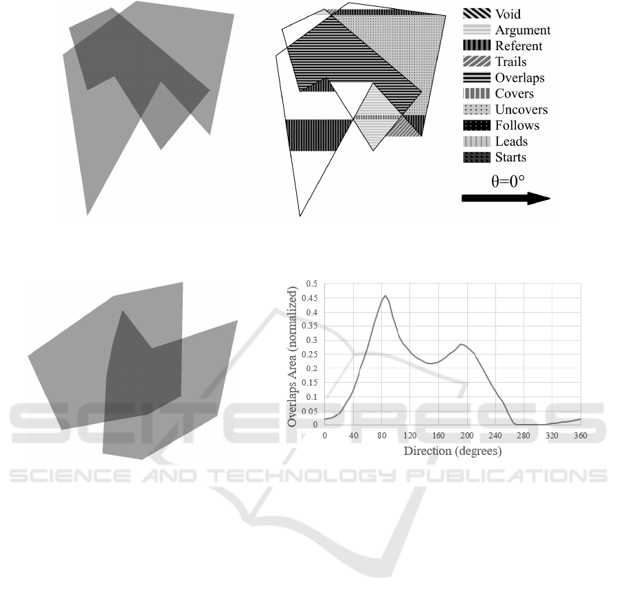
Figure 1: On the left, the original image with two intersecting objects. Areas where the objects overlap are shown in dark grey.
On the right, that image divided into φ-regions in the horizontal left-to-right direction θ. Regions without a corresponding
φ-group are left blank.
Figure 2: On the left, an example pair of objects. Areas where the objects overlap are shown in dark grey. On the right,
a histogram of the area corresponding to the overlaps relation between the two objects in all directions. Area has been
normalized to a percentage of the Region of Interaction, as explained in Sections 2.3.2 and 4.
2.1 Existing RPDs
Many RPDs exist, and have built upon each other over
time. The angle histogram might be the first true
RPD. It is able to model directional relations such
as “to the right of”, “above” etc, (Keller and Wang,
1995) (Keller and Wang, 1996) (Krishnapuram et al.,
1993) (Miyajima and Ralescu, 1994). The force his-
togram generalizes the angle histogram, and also im-
proves upon it (Matsakis and Wendling, 1999). While
the angle and force histograms can model directional
relations, there are others such as the R Histogram
and the Allen Histogram that can model distance or
topological relations (Naeem and Matsakis, 2015).
The recently introduced φ-descriptor (Matsakis et al.,
2015) is the first RPD able to model a variety of di-
rectional, topological, and distance relations (Francis
et al., 2018). In other words, it can describe a larger
set of relations than any other existing RPD. A more
in-depth review of RPDs is available in (Naeem and
Matsakis, 2015).
2.2 The Force Histogram
The force histogram sees objects as physical plates
and determines the sums of forces (like gravitational
forces) exerted by the particles of one object on the
particles of another object. A sum is calculated for
each direction in space. There are algorithms to cal-
culate the force histogram in the case of 2D vector
objects (Recoskie et al., 2012), as well as 3D vector
objects (Reed et al., 2014). In the 2D case, horizon-
tal lines partition the objects into trapezoidal pieces.
The areas of these pieces are determined and used to
calculate the value of the descriptor in the horizontal
direction. The objects are then rotated to the next di-
rection in a direction set, and the process is repeated
for each direction. In the 3D case, planes are used to
intersect the 3D objects into 2D objects, and the 2D
algorithm is applied to the resulting objects.
Computation of the -Descriptor in the Case of 2D Vector Objects
61
2.3 The Phi-descriptor
For each direction in a direction set, the φ-descriptor
algorithm divides the objects into subregions (φ-
regions). Each φ-region corresponds to an elemen-
tary spatial relationship in that direction. The area and
height of each φ-region are determined, and the val-
ues that correspond to the same group of relationships
(φ-group) are summed. The process is repeated in all
directions to form the complete φ-descriptor (see Fig-
ures 1 and 2). The descriptor can be conceptualized
as a set of histograms, one for each φ-group, with the
directions as bins. The value in each bin is an area or
height.
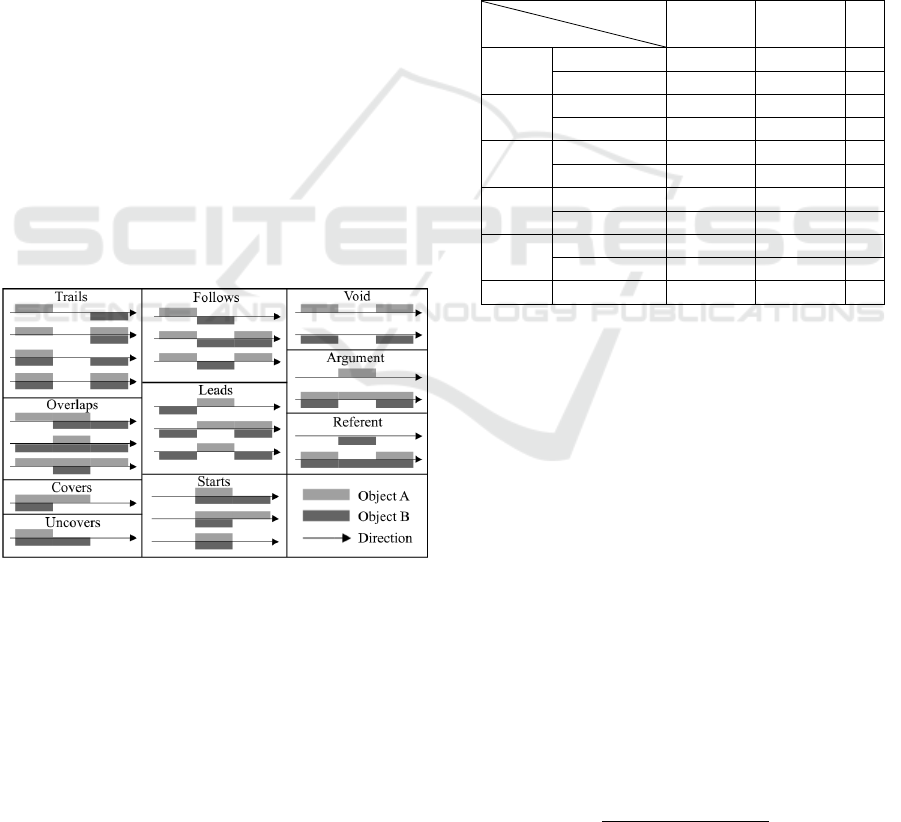
2.3.1 Phi-groups
An important aspect of this algorithm we refer to as
φ-groups. These are groups of elementary spatial re-
lations, each group sharing some characteristic de-
scribed by the verb naming the group. For example,
the overlaps group contains all relations where two
objects overlap one another. The trails group con-
tains all relations where there is a gap between the two
objects, i.e. one object trails behind the other. Each
group, along with the elementary spatial relations that
they consist of, can be seen in Figure 3. One of the
core elements of the algorithm is to find regions, φ-
regions, that correspond to a single φ-group.
Figure 3: Elementary spatial relationships in a given direc-
tion and their corresponding φ-groups. Each spatial rela-
tionship is represented by horizontal slices of two objects A
and B. Slices for different objects have been split apart for
clarity; areas where object A is shown stacked on object B
represent areas where two objects overlap.
2.3.2 φ-Descriptor
The descriptor can be seen as a matrix of numbers, a
column for each direction and a pair of rows for each
φ-group, as seen in Table 1. The pair of rows contain
areas and heights. Each element of the matrix is the
sum of the areas or heights of all φ-regions sharing a
φ-group in a single direction. For example, if there
are two regions with the trails φ-group in direction θ
then the cells for trails in direction θ would contain
one for the sum of the areas, and one for the sum of
the heights. In addition to the φ-groups, the first two
rows of the descriptor show the area and height of the
Region of Interaction in each direction (see Section
3.1). These two values are the sum of the areas and
heights, respectively, of all φ-regions in the direction.
Table 1: An example of part of a φ-descriptor. 72 directions
were tested for this example. Each row represents an ele-
mentary spatial relation (or the Region of Interaction) and
the corresponding sums of areas and heights for each tested
direction. For example, the sum of the areas of the φ-regions
corresponding to the trails φ-group in direction 5
◦
is 10461
(shown below in bolded font).
φ-Group
θ
0
◦
5
◦
...
RoI
area 310009 311138 ...
height 516.681 533.891 ...
Void
area 404 234 ...
height 202 36.137 ...
Arg
area 7769 7819 ...
height 75.062 70.710 ...
Ref
area 7863 9200 ...
height 129.966 120.720 ...
Trails
area 7481 10461 ...
height 124.683 129.641 ...
... ... ... ... ...
2.4 Similarity Measures
Two similarity measures, MinMax and SubAdd, are
used to compare the similarity of φ-descriptors. These
measures have previously been used and detailed in
(Matsakis, 2016) to compare φ-descriptors of pairs of
raster objects. They each require that the descriptors
use the same direction set, and that all values are non-
negative. The values from one descriptor are com-
pared against their counterpart in the other descriptor;
the pair of values d1(θ) and d2(θ) would refer to the
same element in each descriptor (ex. trails area in di-
rection θ).
2.4.1 MinMax Similarity
The MinMax of the two descriptors is essentially the
ratio between the sum of the minima and the sum of
the maxima the pairs of values:
∑
min(d1(θ), d2(θ))
∑
max(d1(θ), d2(θ))
(1)
ICPRAM 2020 - 9th International Conference on Pattern Recognition Applications and Methods
62
The MinMax similarity is 1.0 if both descriptors
are identical, and lower values indicate less similarity.
2.4.2 SubAdd Similarity
The SubAdd of the two descriptors is essentially the
ratio between the sum of the absolute differences and
the sum of the sums of the pairs of values:
1 −
∑
|d1(θ) −d2(θ)|
∑
|d1(θ) +d2(θ)|
(2)
The SubAdd similarity is 1.0 if both descriptors
are identical, and lower values indicate less similarity.
3 ALGORITHM
The φ-descriptor is built upon the principle that pairs
of objects can be divided into regions (φ-regions), for
each direction in a direction set, and these regions
correspond to specific sets of elementary spatial re-
lations (φ-groups). The primary goal then of any φ-
descriptor-based algorithm is to find an appropriate
way to create these regions and identify the spatial
relations they correspond to. Using the areas and
heights of these φ-regions, the descriptor can be built
in one direction; to complete the φ-descriptor, the pro-
cess is repeated in all directions. The goal of this new
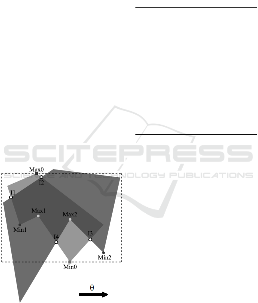
Figure 4: This image shows the Region of Interaction, as a
dotted box, in direction θ. The PoI are shown: Max0 (black
square), Min0 (grey square), Intersections (white circle with
black border), Local Minima (black circle), and Local Max-
ima (grey circle).
algorithm is to calculate the φ-descriptor for a pair of
vector objects; this process is summarized in Algo-
rithm 1.
Algorithm 1: Vector φ-Descriptor Computation.
1: for all θ ∈ direction set do
2: Rotate original objects by −θ.
3: Find vertices of the inputted objects where ele-
mentary spatial relations change, referred to as
Points of Interest (PoI).
4: for all PoI do {Create Rays}
5: Cast horizontal “rays” through the PoI.
6: Determine the points where the ray inter-
sects with the objects (endpoints).
7: Determine PoI φ-groups for directions ”left-
to-right” and ”right-to-left”.
8: Add edges between endpoints closest to PoI.
9: end for
10: Divide the objects into φ-regions based on the
boundaries of the original objects that intersect
the rays.
11: Calculate areas and heights of φ-regions.
12: Save them to descriptor.
13: end for
3.1 Points of Interest
We focus here on the ”left-to-right” direction (or di-
rection θ=0
◦
). For any other direction θ, rotate the
objects by −θ beforehand. To find the φ-regions we
must look at what would make one portion of the ob-
jects change to a different elementary spatial relation-
ship. The points in which these changes occur we
call Points of Interest (PoI) (see Figure 4) and are
confined to the region of interaction, the space which
both objects share in direction θ=0
◦
. The top-most
and bottom-most points of the region of interaction
are both PoI, as well as any local extrema within that
region, and any point where the boundaries of the ob-
jects intersect.
The Region of Interaction is defined by two ver-
tices, Max0 and Min0 (the top-most and bottom-most
points). The extrema are vertices with both neigh-
bours either above (minima), or below (maxima) the
vertex. We consider that a pair of vertices can form
an extrema pair if both vertices share a Y value, they
are neighbours of each other, and their remaining two
neighbours are both either above (minima), or below
(maxima) the pair. After a rotation the set of PoI
which correspond to these two types may change (i.e.
a minima may no longer be a minima after a rotation),
and thus they must be recalculated for each direction.
The intersections are points where an edge from
one object intersects an edge from the other. While
Computation of the -Descriptor in the Case of 2D Vector Objects
63
the other types of PoI may change after each rotation,
the intersections remain the same throughout the algo-
rithm. For this reason, they are calculated only once
in a pre-processing step.
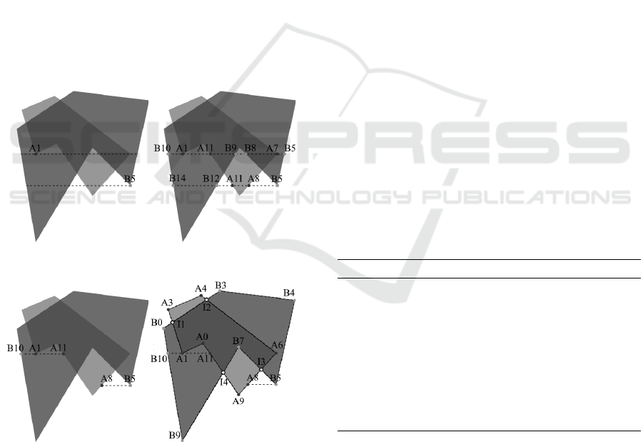
3.2 Rays
At each PoI we pass a horizontal ”ray” and determine
the locations in which it intersects the edges of the two
objects. We call these intersection points endpoints.
We sort the endpoints left to right, and by counting
how many endpoints are on either side of an endpoint
we can determine whether it lies on object A, B, both
or neither; this is the endpoint’s source.
Edges are added between the endpoints along the
ray. These edges serve to divide the objects into φ-
regions based on the changing elementary spatial rela-
tionships (as defined by the PoI). The endpoints along
the top-most and bottom-most rays are all connected
by edges, while intersection and extrema rays only
have edges added directly adjacent to PoI. An exam-
ple of the process to create rays is shown in Figure 5
by creating two rays from local minima.
(a) (b)
(c) (d)
Figure 5: An example creating two rays from local minima.
a) Local minima A1 and B5 along with the rays passing
through. b) All ray intersections located. c) The edges and
endpoints formed by the ray are determined. d) The new
edges (dotted-lines) and endpoints added to the original ob-
jects.
3.3 φ-Regions
While creating the rays, the sources of the endpoints
were determined, and edges added along the ray.
By looking at the sources of an endpoint and its
two neighbouring endpoints, we can determine the φ-
group of the center endpoint. For example, if a point
has the source A, and the neighbouring sources belong
to neither object, we can know (Figure 3) that the end-
point corresponds to the φ-group Argument. Once we
have identified the φ-groups, and all rays have been
created, we can begin forming the φ-regions. To ac-
complish this we traverse the edges above each point
on a ray in a counter-clockwise direction; the φ-region
is the smallest cycle above and to the right that con-
tains the starting endpoint on the ray. As we traverse
the region, we remove the directed edges that form it;
this reduces computation costs for traversing subse-
quent φ-regions.
3.4 φ-Region Areas and Heights
The φ-descriptor requires the size of each φ-region.
The area of the φ-region is used for the size, as well
as the height of the φ-region. Algorithm 2 shows the
process to find the area of a polygon (φ-region) (Page,
2011). To calculate the height of the φ-region, take
the difference of the maximum and minimum Y val-
ues of all points in the φ-region. After the sizes of all
φ-regions are determined for a direction θ, we look
at each φ-region and add the appropriate areas and
heights to the θ and θ+180
◦
columns at the two rows
associated with the φ-groups of the region.
Algorithm 2: Find φ-Region Area.
1: numPoints = number of points in polygon[].
2: area = 0
3: j = numPoints -1
4: for i = 0 to i = numPoints do
5: area+ = (polygon[ j].x + polygon[i].x ) ∗
(polygon[ j].y − polygon[i].y)
6: j = i
7: end for
8: area = area / 2
The φ-descriptor contains the areas and heights of
φ-regions in multiple directions. The number of direc-
tions k must be an even number greater than zero, i.e.,
k = 2 j where j ∈ Z, j ≥ 1. This is because directions
are processed in pairs; when a φ-group in direction
θ is determined the φ-group for direction θ+180
◦
is
easily determined as well.
The objects are rotated about the centroid of the
two objects. We require the centroid of the two ob-
ICPRAM 2020 - 9th International Conference on Pattern Recognition Applications and Methods
64

jects such that they can rotate around the same origin;
this will preserve their relative position. This centroid
is calculated once at the start of the algorithm and
used for each rotation. The x-coordinate of the cen-
troid, for example, is the average of the x-coordinates
of all vertices from both objects.
In addition to rotating, we remove all remaining
points and edges we added when creating the rays.
We want to return the objects to their original state,
i.e., with only the initial vertices, object intersections,
and edges on the boundaries of the objects between
these vertices and intersections.
Algorithm 3: Rotate Object.
1: centroid = (mean(X values), mean(Y values)
2: for all Point p in object do
3: ∆x = p.x − centroid.x
4: ∆y = p.y − centroid.y
5: p.x = centroid.x +∆x ∗ cosθ − ∆y ∗ sinθ
6: p.y = centroid.y + ∆x ∗ sinθ + ∆y ∗ cosθ
7: end for
4 EXPERIMENTS
The testing plan to validate the new algorithm pre-
sented in this paper can be broken into five steps:
1. Generate random vector object pairs.
2. Calculate φ-descriptors of vector object pairs us-
ing the new algorithm.
3. Convert vector object pairs to raster object pairs.
4. Calculate φ-descriptor of raster object pairs using
the existing algorithm.
5. Compare descriptors and processing time.
It is expected that a vector object pair and the
corresponding rasterized object pair should produce
near identical descriptors, and the higher the resolu-
tion of the rasterized objects the higher the similar-
ity between the two descriptors. Note, however, that
the descriptors must first be “normalized” using the
size of the Region of Interaction mentioned in Section
2.3.2. For each direction, each area in the descriptor
is divided by the area of the Region of Interaction,
and each height is divided by the height of the Region
of Interaction. In the end, the normalized descriptors
contain percentages, rather than actual size data; for
example, “trails area in direction θ accounts for 2.1%
of the Region of Interaction area”. When comparing
the descriptors we ask the following question, ”Does
this region account for the same percentage in both
descriptors?”
The random generation of vector object pairs is
briefly discussed in Section 4.1, the results of the ex-
periments are presented in Section 4.2, and the limi-
tations with the algorithm are stated in Section 4.3.
4.1 Test Data
Random vector objects pairs were generated using
Ounsworth’s algorithm (Ounsworth, 2012). A num-
ber of random directions is selected. A point is placed
at a random distance in each direction, maintaining a
clockwise progression. The algorithm contains some
variables to have some control over the output, such
as the number of directions, the center of the poly-
gon, the “average” distance from the center for the
points, the “spikiness” (which determines how much
variance there is from the average distance) and the
“irregularity” (which controls how even the direction
set is). Two examples of randomly generated object
pairs are shown in Figure 6.
Figure 6: Two example object pairs created with the polygon generating algorithm.
Computation of the -Descriptor in the Case of 2D Vector Objects
65
●
●
●
●
●
●
●
●
●
●
●
●
●
●
●
●
●
●
●
●
●
●
●
●
●
●
●
●
●
●
●
●
●
●
●
●
●
●
●
●
●
●
●
●
●
●
●
●
●
●
●
●
●
●
●
●
●
●
●
●
●
●
●
●
●
●
●
●
●
●
●
●
●
●
●
●
●
●
●
●
●
●
●
●
●
●
●
●
●
●
●
●
●
●
●
●
●
●
●
●
●
●
●
●
●
●
●
●
●
●
●
●
●
●
●
●
●
●
●
●
●
●
●
●
●
●
●
●
●
●
●
●
●
●
●
●
●
●
●
●
●
●
●
●
●
●
●
●
●
●
●
●
●
●
●
●
●
●
●
●
●
●
●
●
●
●
●
●
●
●
●
●
●
●
●
●
●
●
●
●
●
●
●
●
●
●
●
●
●
●
●
●
●
●
●
●
●
●
●
●
●
●
●
●
●
●
●
●
●
●
●
●
●
●
●
●
●
●
●
●
●
●
●
●
●
●
●
●
●
●
●
●
●
●
●
●
●
●
●
●
●
●
●
●
●
●
●
●
●
●
●
●
●
●
●
●
●
●
●
●
●
●
●
●
●
●
●
●
●
●
●
●
●
●
●
●
●
●
●
●
●●
●
●
●
●
●
●
●
●
●
●
●
●
●
●
●
●
●
●
●
●
●
●
●
●
●
●
●
●
●
●
●
●
●
●
●
●
●
●
●
●
●
●
●
●
●
●
●
●
●
●
●
●
●
●
●
●
●
●
●
0.25
0.50
0.75
1.00
100 300 500 700 900 1100 1300 1500 1700 1900
Image Width (Pixels)
MinMax Similarity
Function
Height
Area
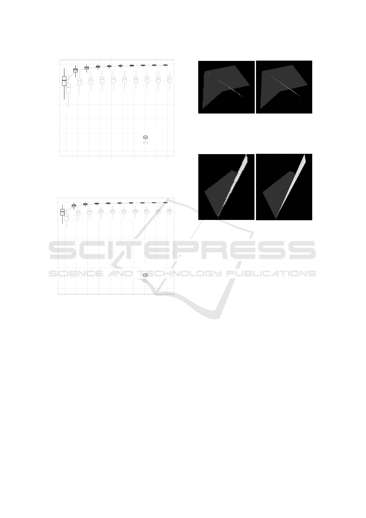
Figure 7: Results of the MinMax similarity tests over vari-
ous resolutions. 300 object pairs were tested at each resolu-
tion. As the resolution increases, the similarity improves.
●
●
●
●
●
●
●
●
●
●
●
●
●
●
●
●
●
●
●
●
●
●
●
●
●
●
●
●
●
●
●
●
●
●
●
●
●
●
●
●
●
●
●
●
●
●
●
●
●
●
●
●
●
●
●
●
●
●
●
●
●
●
●
●
●
●
●
●
●
●
●
●
●
●
●
●
●
●
●
●
●
●
●
●
●
●
●
●
●
●
●
●
●
●
●
●
●
●
●
●
●
●
●
●
●
●
●
●
●
●
●
●
●
●
●
●
●
●
●
●
●
●
●
●
●
●
●
●
●
●
●
●
●
●
●
●
●
●
●
●
●
●
●
●
●
●
●
●
●
●
●
●
●
●
●
●
●
●
●
●
●
●
●
●
●
●
●
●
●
●
●
●
●
●
●
●
●
●
●
●
●
●
●
●
●
●
●
●
●
●
●
●
●
●
●
●
●
●
●
●
●
●
●
●
●
●
●
●
●
●
●
●
●
●
●
●
●
●
●
●
●
●
●
●
●
●
●
●
●
●
●
●
●
●
●
●
●
●
●
●
●
●
●
●
●
●
●
●
●
●
●
●
●
●
●
●
●
●
●
●
●
●
●
●
●
●
●
●
●
●
●
●
●
●
●
●
●
●
●
●
●
●
●
●
●
●
●
●
●
●
●
●
●
●
●
●●
●
●
●
●
●
●
●
●
●
●
●
●
●
●
●
●
●
●
●
●
●
●
●
●
●
●
●
●
●
●
●
●
●
●
●
●
●
●
●
●
●
●
●
●
●
●
●
●
●
●
●
●
●
●
●
●
●
●
●
●
●
0.4
0.6
0.8
1.0
100 300 500 700 900 1100 1300 1500 1700 1900
Image Width (Pixels)
SubAdd Similarity
Function
Height
Area
Figure 8: Results of the SubAdd similarity tests over various
resolutions. 300 object pairs were tested at each resolution.
As the resolution increases, the similarity improves.
4.2 Results
Three hundred vector object pairs were created, con-
verted to raster pairs with various resolutions, and
tested against both the raster and vector φ-descriptor
algorithms. Figures 7 and 8 show the MinMax and
SubAdd similarity results. The similarities tend to im-
prove as the resolution of the raster objects increases.
The graphs of the results show some outliers for
pairs of descriptors that are particularly dissimilar.
These results are from images that have very small
regions, as shown in Figures 9 and 10. When rasteriz-
ing φ-regions that are very thin, portions of the objects
may fit between rows or columns of pixels; the result-
ing raster image may not show any pixels for these
Figure 9: These are two raster images of object pair 73. The
image on the left has a width of 100 pixels, and the image
on the right 1,100. The image on the left shows gaps in the
thin object, which was too thin to be correctly rasterized. It
therefore produced a very low similarity score.
Figure 10: These are two raster images of object pair 43.
The image on the left has a width of 100 pixels, and the
right 1,100. There are multiple locations in the left image
where a pixel from object A is directly adjacent to a pixel
from object B. However, this never actually occurs in the
vector image, as there is either an overlap or a space be-
tween the object. The left image therefore produced a very
low similarity score.
regions at all, as shown in Figure 9. When objects
have edges that are very close, the raster image may
have pixels from the two objects directly adjacent,
while the vector image shows the objects to overlap,
or have a gap, as shown in Figure 10. It is also im-
portant to note that we are not comparing the original
descriptors, but rather the normalized descriptors, as
explained in Section 4. If we look at Figure 9 it is
apparent that the region of interaction will change de-
pending on what pixels are detected for each object.
While these outliers show poor similarity, this
does not indicate that either algorithm is producing
incorrect results. Both algorithms are giving the cor-
rect results for the input data provided.
When analysing the time required to calculate the
φ-descriptor we must consider the number of vertices
in the vector object. Figure 11 shows the processing
time for 100 randomly generated object pairs, with
random numbers of vertices (the total number of ver-
tices of the pairs ranges from 12 − 181). We can see
that the number of vertices has a large impact on the
processing time; Figure 12 shows the object pair that
required the most processing time, and had the most
vertices.
ICPRAM 2020 - 9th International Conference on Pattern Recognition Applications and Methods
66
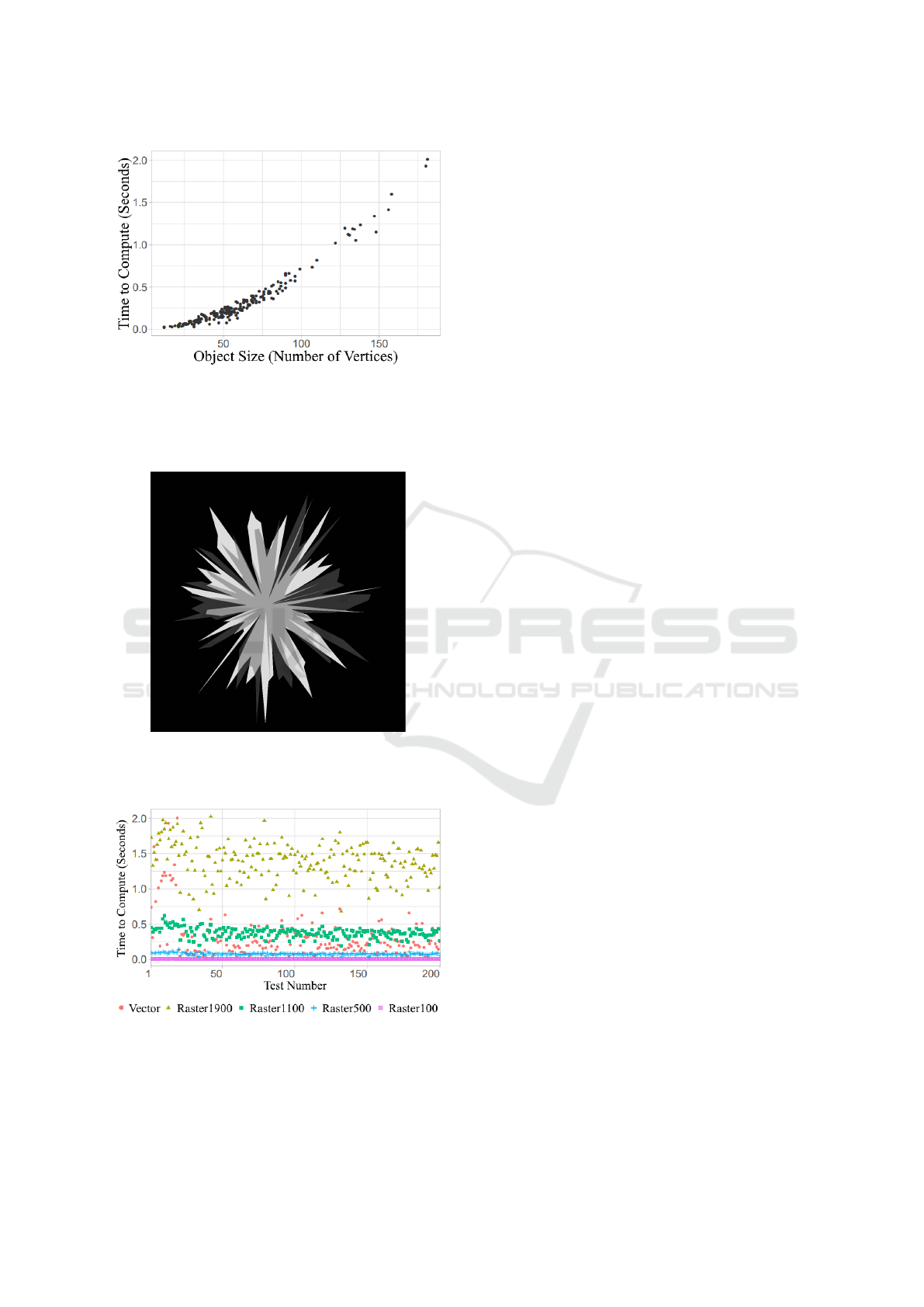
Figure 11: The processing times of 100 vector object pairs.
The number of vertices refers to the sum of number of ver-
tices of both objects in each pair. It is clear that a larger
number of vertices increases the processing time of the φ-
descriptor computation for vector objects.
Figure 12: The vector object pair that required the most
processing time. There are a total of 181 vertices between
the two objects.
Figure 13: A comparison of the processing times of 100
pairs of objects. We consider vector objects, and raster ob-
jects with a pixel width of 100, 500, 1100, and 1900.
Figure 13 compares the processing time of
these same 100 vector object pairs to their raster
counterparts. We examine the raster objects at
100, 500, 1100, and 1900 pixels in width. We see
the computation time for the φ-descriptor of raster
objects is very consistent for a given object size, and
as expected the more pixels in the raster object, the
more processing time is required. When the raster
objects are between 500 and 1100 pixels in width,
and the vector object pair has less than 100 vertices,
the φ-descriptors are often processed in roughly the
same time range.
4.3 Current Limitations
There are some limitations with the algorithm in re-
gard to the current implementation that should be
noted. In particular, the handling of objects with holes
or made of multiple connected components has not
been implemented. It should be noted that these limi-
tations are not a fault of the algorithm itself, but rather
is a fault of how it was implemented. Work is cur-
rently being done to eliminate these limitations and to
test robustness of the algorithm against these cases.
5 CONCLUSION
We have introduced the first algorithm to calculate the
φ-descriptor in the case of 2D vector objects. Our mo-
tivation was to show that the φ-descriptor is a capable
successor to a well-known Relative Position Descrip-
tor (the force histogram), and is equally versatile. The
algorithm was tested against 300 randomly generated
pairs of 2D vector objects. Each pair had the 2D vec-
tor φ-descriptor computed using the new algorithm,
the corresponding 2D raster φ-descriptor was com-
puted as well, and the two descriptors were compared.
Our results have shown that in most cases the vector
and raster descriptors were very similar as expected,
and the higher the resolution of the rasterized objects
the higher the similarity. Cases with poor similarity
were found to have very thin regions that could not be
properly rasterized, i.e., the low similarity scores were
due to data loss in the conversion, not a fault of either
algorithm. Potential applications of this work are in
areas where a powerful RPD is required to encapsu-
late a great amount of spatial relationship information
between 2D vector objects (e.g., human-robot com-
munication and geographical information systems).
Work is currently being done to eliminate the lim-
itations discussed in Section 4.3. Future versions of
this algorithm are planned to be capable of handling
objects with holes or made of multiple connected
Computation of the -Descriptor in the Case of 2D Vector Objects
67

components. This algorithm also has the potential to
be expanded to the case of 3D vector objects.
REFERENCES
Francis, J., Rahbarnia, F., and Matsakis, P. (2018). Fuzzy
nlg system for extensive verbal description of rela-
tive positions. 2018 IEEE International Conference
on Fuzzy Systems (FUZZ-IEEE), pages 1–8.
Freeman, J. (1975). The modelling of spatial relations.
Computer graphics and image processing, 4(2):156–
171.
Keller, J. M. and Wang, X. (1995). Comparison of spatial
relation definitions in computer vision. In Proceed-
ings of 3rd International Symposium on Uncertainty
Modeling and Analysis and Annual Conference of the
North American Fuzzy Information Processing Soci-
ety, pages 679–684. IEEE.
Keller, J. M. and Wang, X. (1996). Learning spatial rela-
tionships in computer vision. In Proceedings of IEEE
5th International Fuzzy Systems, volume 1, pages
118–124. IEEE.
Krishnapuram, R., Keller, J. M., and Ma, Y. (1993). Quan-
titative analysis of properties and spatial relations of
fuzzy image regions. IEEE Transactions on fuzzy sys-
tems, 1(3):222–233.
Matsakis, P. (2016). Affine properties of the relative posi-
tion phi-descriptor. In 2016 23rd International Con-
ference on Pattern Recognition (ICPR), pages 1941–
1946.
Matsakis, P., Naeem, M., and Rahbarnia, F. (2015). In-
troducing the phi-descriptor - a most versatile relative
position descriptor. In ICPRAM, pages 87–98.
Matsakis, P. and Wendling, L. (1999). A new way to repre-
sent the relative position between areal objects. IEEE
Transactions on pattern analysis and machine intelli-
gence, 21(7):634–643.
Miyajima, K. and Ralescu, A. (1994). Spatial organization
in 2d segmented images: representation and recogni-
tion of primitive spatial relations. Fuzzy Sets and Sys-
tems, 65(2-3):225–236.
Naeem, M. and Matsakis, P. (2015). Relative position de-
scriptors - a review. ICPRAM 2015 - 4th International
Conference on Pattern Recognition Applications and
Methods, Proceedings, 1:286–295.
Ounsworth, M. (2012). Algorithm to generate random
2d polygon: https://stackoverflow.com/questions/
8997099/algorithm-to-generate-random-2d-polygon.
Page, J. D. (2011). Algorithm to find the area of a polygon:
https://www.mathopenref.com/coordpolygonarea2.
html.
Recoskie, D., Xu, T., and Matsakis, P. (2012). A general al-
gorithm for calculating force histograms using vector
data. In ICPRAM (1), pages 86–92.
Reed, J., Naeem, M., and Matsakis, P. (2014). A first algo-
rithm to calculate force histograms in the case of 3D
vector objects. pages 104–112.
Santosh, K., Lamiroy, B., and Wendling, L. (2012). Symbol
recognition using spatial relations. Pattern Recogni-
tion Letters, 33:331–341.
ICPRAM 2020 - 9th International Conference on Pattern Recognition Applications and Methods
68
