Efﬁcient Visualization and Set-theoretic Difference Operations for

Accurate Geometric Modeling in Real-time Simulations

Alexander Leutgeb

, Michael Florian Hava

and Alexander Hans Leitner

Unit Industrial Software Applications, RISC Software GmbH, Softwarepark 35, Hagenberg, Austria

Keywords:

Implicit Representation, Point Cloud Fitting, Set-theoretic Modeling, Ray Casting, Real-time Simulation.

Abstract:

We present a novel approach, which supports efﬁcient visualization and set-theoretic difference operations for

accurate geometric modelling in real-time simulations. The geometric operands can be in any representation

as long as they are watertight and are convertible to an oriented point cloud. A novel region growing based

ﬁtting routine converts the oriented point clouds into a watertight piecewise quadratic implicit representation.

During set-theoretic modeling these implicit representations are mapped to the ﬁxed depth hierarchical grid

of the resulting geometric model. Thereby a surface elimination algorithm removes parts not contributing

to the ﬁnal surface. This guarantees that the number of already performed modeling operations have only a

minor performance impact on the algorithms processing the model. For visualization a novel ray casting based

approach was developed, enabling interactive frame rates at Full-HD screen resolutions. The evaluation of the

developed method proves its modeling performance and high geometric accuracy by means of the simulation

of subtractive manufacturing examples.

1 INTRODUCTION

There is a strong need for an efﬁcient visualization

and set-theoretic difference operations in the context

of accurate geometric modeling in real-time simu-

lations. For example, the simulation of subtractive

manufacturing - material removal processes, such as

milling, turning or drilling - have become complex

tasks, requiring efﬁcient systems for their geometric

model computation and visualization. The complex

multi-axis milling processes result in workpieces with

a high-quality surface ﬁnish requiring manufacturing

tolerances up to 0.001 mm generated by thousands of

removal steps.

Conventional solid modeling systems build the

foundation for computer-assisted geometric design

of “Virtual Products” via Computer Aided Design

(CAD) software. These systems are implemented

with respect to modeling capabilities, geometric mod-

eling precision, exchangeability of geometric for-

mats between different CAD systems, a geometric

representation, which is adequate for further anal-

ysis in the ﬁelds of Computer-Aided Engineering

https://orcid.org/0000-0001-8934-4501

https://orcid.org/0000-0002-5085-1490

https://orcid.org/0000-0002-4081-2586

(Finite-Element-Analysis and Computational-Fluid-

Dynamics). Their modeling operations do not offer

the necessary performance to support the application

in real-time simulations.

Our approach is a geometric modeling sys-

tem, which supports efﬁcient visualization and set-

theoretic difference operations for accurate geomet-

ric modelling in real-time simulations. Thereby the

number of already performed set-theoretic difference

operations has only a minor performance impact

on the algorithms processing the geometric model.

The obtainable precision of the resulting geometric

model matches the requirements of industrial applica-

tions. The algorithms of the system utilize the paral-

lelization potential of modern hardware architectures.

Summarizing, the novelties introduced in this work

are mainly:

• A region growing based ﬁtting routine for ori-

ented points clouds with an implicit representa-

tion using piecewise quadratic functions. The re-

sulting representation is watertight.

• A ﬁxed depth hierarchical grid with an efﬁcient

elimination strategy during set-theoretic modeling

operations.

• An efﬁcient ray casting based visualization sup-

porting interactive frame rates.

Leutgeb, A., Hava, M. and Leitner, A.

Efﬁcient Visualization and Set-theoretic Difference Operations for Accurate Geometric Modeling in Real-time Simulations.

DOI: 10.5220/0008983802990306

In Proceedings of the 15th International Joint Conference on Computer Vision, Imaging and Computer Graphics Theory and Applications (VISIGRAPP 2020) - Volume 1: GRAPP, pages

299-306

ISBN: 978-989-758-402-2; ISSN: 2184-4321

299

2 RELATED WORK

Implicit surfaces are mostly deﬁned by polynomials,

of which Quadrics are the most prominent represen-

tatives (Menon, 1996). These are polynomials of de-

gree two, which in contrast to polynomials of higher

degree, have closed and efﬁcient solutions for certain

geometric problems like intersection computations.

Distance functions d(p) are special functions from R

to R, these compute the distance to the nearest point

on the implicit surface deﬁned via d(p) = 0 for each

point p ∈ R

(Diener, 2012). Signed distance func-

tions (SDF) compute the signed distance, in which

negative distances usual represent the inside of an ob-

ject. In contrast to general implicit functions, dis-

tance functions offer several advantages considering

the simplicity of several computations, like surface

normals (normalized gradient d(p)) and set-theoretic

operations.

2.1 Discrete Signed Distance Fields

Adaptively sampled distance ﬁelds (ADF) use an Oc-

tree for hierarchical space decomposition and each

cell stores at its eight corner positions the discretized

values of a signed distance function (Frisken et al.,

2000). The hierarchical subdivision follows the shape

of the object according to a deﬁned approximation er-

ror. Because of this adaptivity, complex geometric

objects can be represented in a memory efﬁcient way.

This approach enables an efﬁcient computation of the

set-theoretic operations union, intersection, and dif-

ference. One prominent method for the visualization

of adaptively sampled distance ﬁelds is Sphere Trac-

ing. The work of (Bastos and Celes, 2008) represents

an efﬁcient implementation on Graphics Processing

Units (GPUs).

OpenVDB (Museth, 2013) supports a hierarchi-

cal data structure for the efﬁcient representation of

sparse, time-varying volumetric data discretized on

a 3D grid. These values can be of scalar (signed

distance ﬁeld) or vector (velocity vector ﬁeld) type.

In contrast to an Octree, where the branching fac-

tor per dimension is two and its depth determines

the precision, OpenVDB uses a tree structure with a

ﬁxed depth, and the precision depends on the branch-

ing factor per dimension at each hierarchical level.

An Octree based approach has a higher memory ef-

ﬁciency because of better adaptivity to the geometric

shape, but has higher run-times for searching speciﬁc

cells and set-theoretic modeling operations. Besides

the simulation of time-varying changes of volumes,

OpenVDB also supports efﬁcient set-theoretic mod-

eling.

The approaches in this section have the following

limitation: In order to reach a high modeling accuracy

the size of the leaf cells has to be very ﬁne. This ﬁne

granularity has a negative performance impact on set-

theoretic modeling operations.

2.2 Continuous Signed Distance

Functions

Multi-level partition of unity (MPU) implicits sup-

port an adaptive error-driven approximation of a sur-

face via signed distance functions in a precise and fast

way (Ohtake et al., 2003). In order to create the im-

plicit representation, the geometric object (in the con-

crete case deﬁned via an oriented point cloud) is spa-

tial subdivided according to an Octree structure. In

each Octree cell a piecewise quadratic function (lo-

cale shape function) is created, which approximates

the geometry assigned to the according cell. These

shape functions behave like signed distance functions

and yield a value close to zero in the proximity of

the surface of the approximated geometric shape, a

positive value inside and a negative value outside.

In the case, the local shape function exceeds a de-

ﬁned approximation error for the cell assigned geo-

metric object, the ﬁtting routine subdivides the cell

further and performs the approximation on the new

child cells. The algorithm repeats this process until

the approximation error falls below a deﬁned thresh-

old. Locale shape functions are generic Quadrics, bi-

variate Quadrics and their set-theoretic combination.

By this distinction, it is possible to approximate ﬂat

surfaces as well as surfaces with geometric features

like corners and edges at a high precision. The usage

of signed distance functions enables shape blending,

offsetting, and set-theoretic operations like union, in-

tersection, and difference. Visualization methods for

MPU implicits are direct rendering in polygonised

form or Sphere Tracing (Hart, 1996). Because the

MPU approach offers set-theoretic modeling by com-

bining two distinct geometric objects at the time of

visualization, it does not scale with increasing num-

ber of set-theoretic operations.

Sparse low-degree implicits (SLIM) is a method

approximating the surface of a geometric object with

surface elements (Surfel) (Ohtake et al., 2005). The

geometric object is in form of a point cloud. The

deﬁnition of a Surfel consists of a sphere (speciﬁed

via center and radius), and a function approximating

the surface inside the sphere. Functions can be linear,

quadratic or cubic polynomials. The global surface

results from overlapping Surfels and is not continu-

ous. Surface continuity is guaranteed during visual-

ization via ray casting. The construction of the Surfel

GRAPP 2020 - 15th International Conference on Computer Graphics Theory and Applications

300

representation happens in a hierarchical way, by start-

ing with Surfels with a big radius. Depending on a

cost function, which considers the approximation er-

ror and memory efﬁciency the ﬁtting routine further

subdivides these Surfels into ﬁner ones. The SLIM

approach has the problem, in order to represent ge-

ometric features like edges or corners with high ge-

ometric accuracy the subdivision of the Surfels must

be very ﬁne.

3 GEOMETRIC

REPRESENTATION

Our implicit representation is based on the work of

(Ohtake et al., 2003) and supports the following kinds

of local ﬁtted functions inside a support sphere:

• A bivariate quadratic polynomial in local coordi-

nates.

• A piecewise quadratic surface that ﬁts an edge or

a corner.

3.1 Point Cloud Generation

The newly developed geometric modeling method re-

quires a watertight implicit representation of the geo-

metric objects involved in set-theoretic modeling op-

erations. In order to obtain the implicit representation

for a given triangle mesh, it is ﬁrst converted into an

oriented point cloud with a speciﬁed uniform point

density ρ. For each triangle of the input mesh points

are generated:

• Triangle vertices: For each triangle vertex a point

is generated.

• Triangle edges: If a triangle edge width length l

is longer than ρ, then the edge is split into dl/ρe

parts and points are generated between neighbour-

ing parts.

• Triangle area: The longest edge of a triangle

forms the base vector. The height vector is or-

thogonal to the base vector and its magnitude rep-

resents the triangle height. The base and height

vector form a Cartesian coordinate system, in

which an algorithm generates at regular ρ posi-

tions points in both dimensions, but only if the

point is enclosed by the triangle.

For each generated point the surface normal at its

position is computed. Points shared by multiple tri-

angles with different face normals are replicated with

the respective normal.

3.2 Overall Fitting Procedure

For the region growing based approximation of the

oriented point cloud P the metric ρ(P) is introduced.

As the radius of the support sphere during ﬁtting is at

least 2ρ, it is guaranteed that the number of points is

sufﬁcient for ﬁtting the local shape function.

ρ(P) = max

a∈P

( min

b∈P∧a6=b

(ka − bk)) (1)

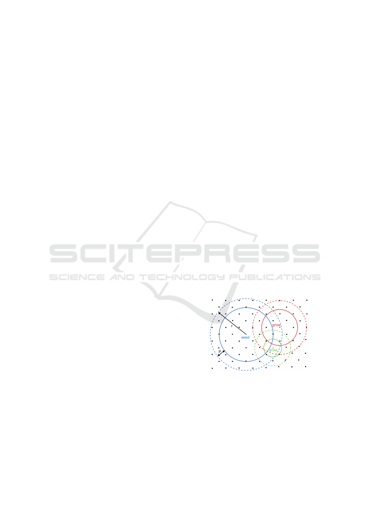
The region growing approach starts with a seed-

ing phase. Thereby the algorithm chooses a random

not already approximated point from the overall point

cloud as center for an initial support sphere with ra-

dius 4ρ. In the case of a successful ﬁt with a lo-

cal function, the algorithm shrinks the support sphere

with radius r by ρ. The space between the initial and

the shrunken sphere is the boundary region (see Fig-

ure 1). All points inside the shrunken support sphere

are considered as approximated. Now the growing

phase begins and the algorithm adds points not al-

ready approximated from this boundary region to the

set of growing points. Now a new center for a new

initial support sphere with radius 4ρ is chosen from

this set of growing points. After a successful ﬁt in-

side the newly created support sphere, the not ap-

proximated points from the new bounding region ex-

tend the set of the growing points. Points considered

as approximated are removed from the set of grow-

ing points. Region growing continues until there are

no more growing points left. If there are any non-

approximated points left, the two stage ﬁtting process

starts again.

Figure 1: Feeding and growing stages.

For each cluster the ﬁtting with local functions

is performed yielding individual bivariate quadratic

polynomials. If the approximation error exceeds the

deﬁned error threshold, the algorithm shrinks the sup-

port sphere by a factor of 0.85 and local function ﬁt-

ting starts again. If the radius gets smaller than 2ρ

ﬁtting is not possible at all.

The overall region growing algorithm works in

parallel in the following way. First the oriented point

Efﬁcient Visualization and Set-theoretic Difference Operations for Accurate Geometric Modeling in Real-time Simulations

301

cloud is placed into a regular grid with cell size 4ρ per

dimension. The grid is partitioned into n work slices

along the dimension with the highest spatial extent,

where n is two times the number of logical processors.

The minimum slice thickness of two times the cell

size prevents race conditions during parallel code ex-

ecution. The parallel region growing algorithm works

in two phases:

• Phase 1: Each logical processor executes the re-

gion growing algorithm inside work slices with an

even sequence number.

• Phase 2: Each logical process executes the region

growing algorithm inside work slices with an odd

sequence number.

The result of the algorithm is a watertight approx-

imation of the oriented point cloud with overlapping

support spheres and local functions.

4 GEOMETRIC MODELING

4.1 Hierarchical Space Decomposition

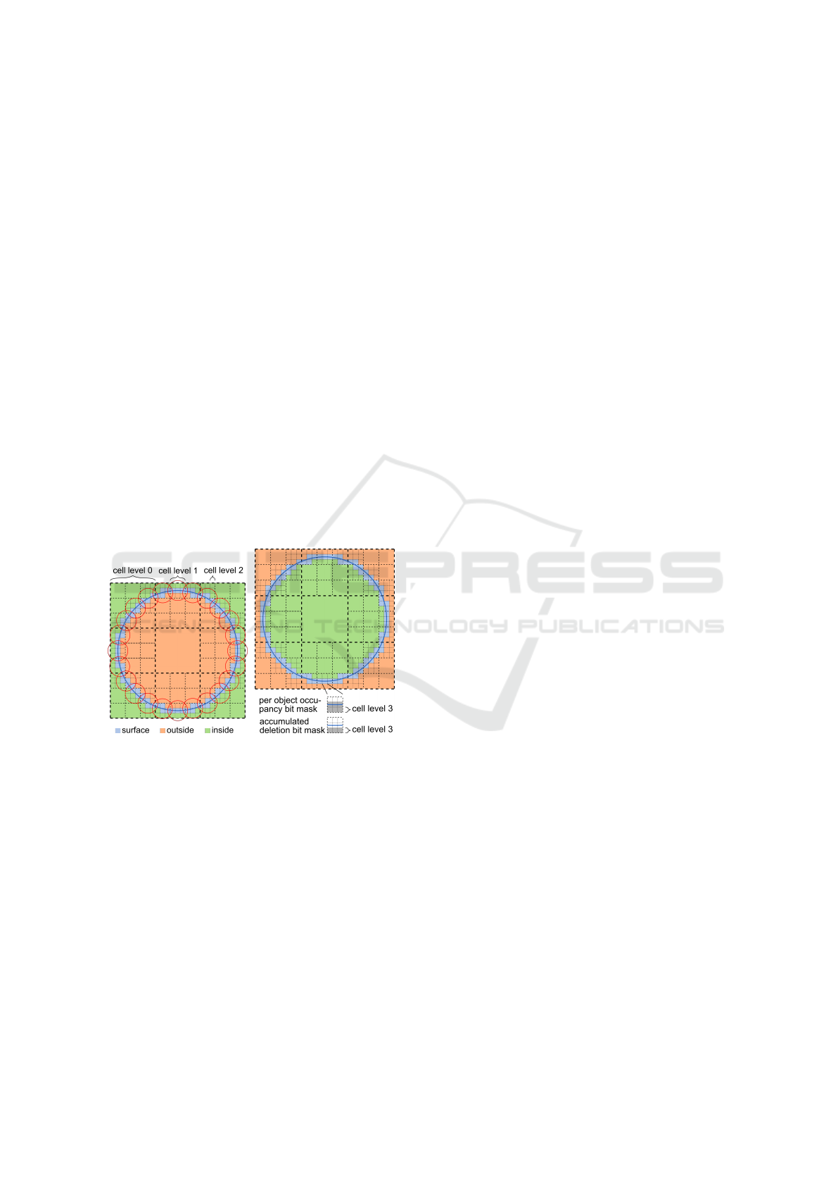
(a) (b)

Figure 2: (a) Grid occupancy of ﬁrst set-theoretic differ-

ence operand (support spheres are red and local functions

are blue). (b) Modeling grid after set-theoretic difference

operation.

During set-theoretic modeling the geometric operand

represented by support spheres with their local

functions is mapped to a hierarchical grid with a

ﬁxed depth (see Figure 2). The developed space-

partitioning scheme is similar to OpenVDB (Museth,

2013) and shares the same advantages (see section

2.1). The cells of the grid can have the classiﬁca-

tions inside, outside or surface. By convention the

initial geometric object is considered as the ﬁrst set-

theoretic difference operand and therefore its surface

orientation is inverted (see Figure 2 (a)) and the initial

modeling grid is completely inside. Surface classiﬁ-

cation can only occur on cell level 2, whereas the clas-

siﬁcations inside and outside can also occur on higher

cell levels. The mapping of the surface represented

via the support spheres with their local functions to

cells works as following. The algorithm checks each

support sphere if it overlaps with cells at cell level 0.

If this is the case, it checks the overlap for each child

cell at the next cell level. It repeats this procedure un-

til cell level 2 is reached. Section 4.2 explains check-

ing for actual surface contribution of a support sphere

with its local function on cell level 2. The ﬁnest cell

level 3 stores a per geometric object grid occupancy

bit mask and an accumulated deletion bit mask. The

mapping logic for cell level 3 is the same as for cell

level 2. Section 4.3 explains the usage of cell level 3

in the context of surface elimination.

4.2 Cell Classiﬁcation

Surface Cells. A support sphere and its local function

are only assigned to a cell on level 2, if there actually

is a surface contribution inside the cell. The surface

contribution is computed in the following way. At

ﬁrst the algorithm computes the axis aligned bound-

ing box (overlap box) resulting from the overlap be-

tween the support sphere and the cell. If the function

has a surface contribution inside the cell it must cross

at least one of the six faces of the overlap box. In

Figure 3 you see one face of the overlap box colored

green. The red circle marks the intersection between

the support sphere and a face plane. The blue curve

marks the intersection between the local function and

the face plane. The green ﬁlled circles mark the posi-

tions, where the signed distance function is evaluated,

and contain the sign of the value. In the case this po-

sition is outside the support sphere, the green ﬁlled

circles are empty. In Figure 3 (a) to (c) you see the

recursive subdivision scheme of the algorithm, which

stops depending on the following cases:

• There are sign changes between neighboring eval-

uation points so the function crosses the space

between these two points and we have a surface

contribution inside the cell. The reference point

(ﬁlled red circle) is the intersection between a line

ranging between these two points and the local

function.

• The size in both dimensions of the subdivided

rectangular areas falls under a certain threshold so

no surface contribution was detected.

The reference point is needed for inside/outside calcu-

lation during visualization via ray casting (see section

5.2).

GRAPP 2020 - 15th International Conference on Computer Graphics Theory and Applications

302

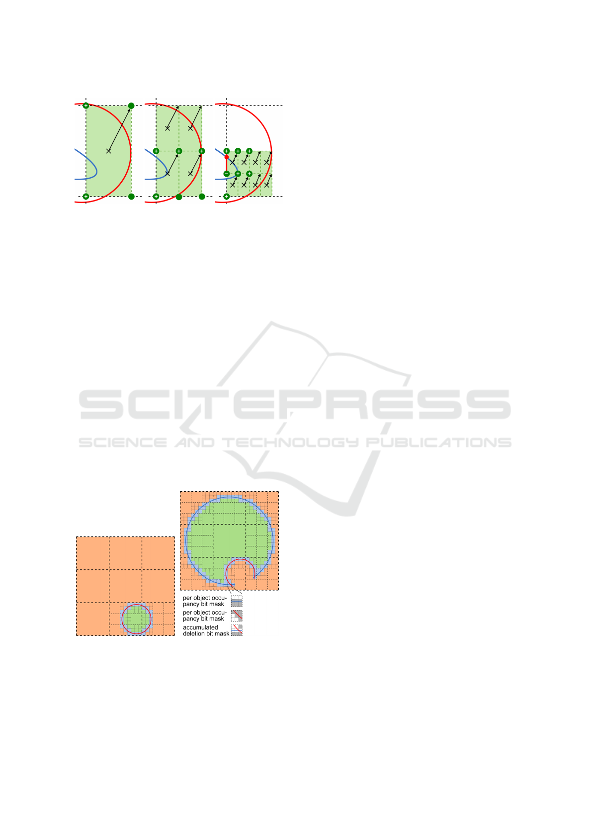
(a) (b) (c)

Figure 3: Determination of surface contribution for local

function. (a) Initial area. (b) Areas after ﬁrst subdivision.

Inside/Outside Cells. The classiﬁcation algorithm

categorizes the non-surface cells into inside or outside

cells in the following three ways, sorted by increasing

computational costs:

1. Adopt the classiﬁcation of direct neighboring cell.

2. If cell center is inside a support sphere evaluate

the according signed distance function for the po-

sition and derive classiﬁcation from sign of result.

3. If cell center is outside of any support sphere, cre-

ate a line ranging from the cell center to the cen-

ter of the closest support sphere. Compute the in-

tersection point between the line and the support

sphere. Evaluate signed distance function for in-

tersection position and derive classiﬁcation from

sign of result.

4.3 Surface Elimination

(a) (b)

Figure 4: (a) Grid occupancy of second set-theoretic differ-

ence operand. (b) Modeling grid after set-theoretic differ-

ence operation showing surface elimination.

Figure 4 illustrates the process of surface elimina-

tion. (a) shows the grid occupancy of the second set-

theoretic difference operand. In (b) you see the mod-

eling grid after the set-theoretic difference operation,

where all the surface cells of the initial geometric ob-

ject inside the surface cells of the set-theoretic differ-

ence operand were cleared. Clearing in this context

means removing all surfaces from surface cells and

changing the cell classiﬁcation from surface to out-

side. If all child cells of a parent cell have the same

cell classiﬁcation outside, then the subdivision of the

parent cell into child cells is withdrawn and the algo-

rithm transfers the child cell classiﬁcation to the par-

ent cell. Additional surface elimination can occur by

using the information from cell level 3. Thereby we

have to differentiate between two different cases:

• If all the bits in the accumulated deletion bit mask

are set, then all surfaces from the surface cell are

removed and the cell classiﬁcation is changed to

outside.

• If for all the set bits of the per object occupancy bit

mask the according bits in the accumulated dele-

tion bit mask are set, then the surface of the geo-

metric object can be removed.

5 VISUALIZATION

5.1 Ray Casting of Watertight Surfaces

For the visualization of surfaces resulting from set-

theoretic modeling ray casting was ﬁrst mentioned in

the work of (Roth, 1982). Thereby the operands in-

volved during modeling must be in watertight form.

The basic idea is to calculate the surface intersec-

tions of all involved geometrics objects with the ray.

Then the algorithm sorts the intersections according

to an increasing distance between ray origin and in-

tersections. Now the algorithm calculates the result-

ing surface point in the following way. It starts with a

counter initialized with a predeﬁned value. By going

through the list of intersections it decrements or in-

crements this counter depending on the fact if a ray

enters respectively leaves a geometric object at the

current intersection. The method detects entering or

leaving by using the surface normal at the intersection

point and the normalized ray direction. If the normal-

ized ray direction points into the same half-space as

the surface normal the ray leaves the geometric ob-

ject, otherwise the ray enters it. If during counting the

counter reaches a deﬁned value the resulting surface

point is hit. This visualization principle is also appli-

cable to the developed surface representation, because

overlapping support spheres with local functions de-

scribe a watertight surface of a geometric operand.

Efﬁcient Visualization and Set-theoretic Difference Operations for Accurate Geometric Modeling in Real-time Simulations

303

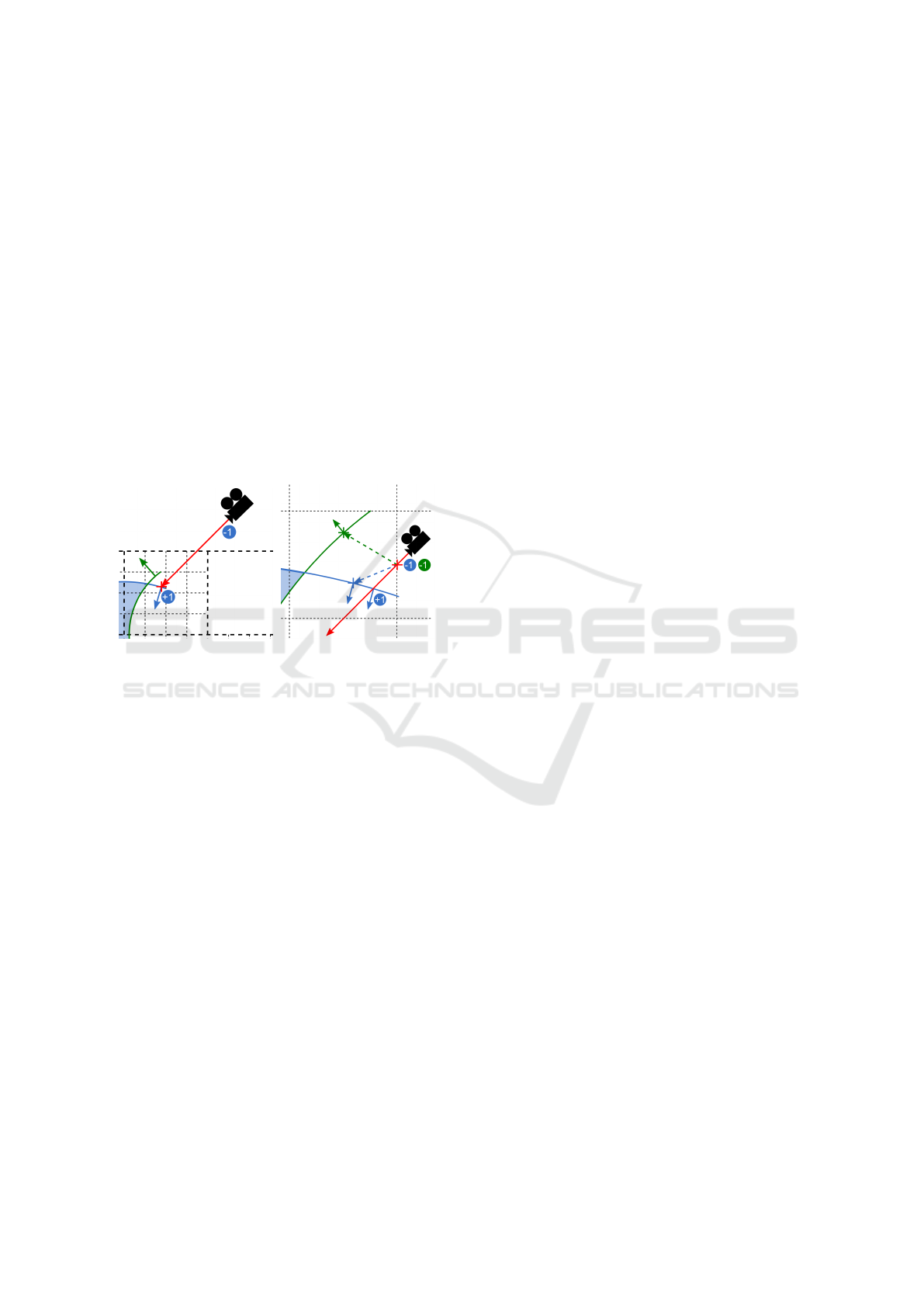
5.2 Ray Casting of Non-watertight

Surfaces

Because of the surface elimination during set-

theoretic modeling we lose the watertightness of the

geometric operands. In Figure 5 (a) you see the grid

occupancy in the case of a set-theoretic difference op-

eration where the initial geometry is colored blue and

the subtractive geometry is colored green. By conven-

tion, we deﬁne the initial geometric object as ﬁrst sub-

tractive geometric object. Therefore the counter at the

ray origin is initialized with -1 (ray origin inside ini-

tial geometric object). During counting, the algorithm

reaches the resulting surface point, if the counter gets

the value 0. If we execute the usual counting proce-

dure, the resulting surface point will be wrong, be-

cause of the missing ray intersections between the ray

and the geometric objects.

(a) (b)

Figure 5: (a) Wrong resulting surface point (red cross ) dur-

ing counting. (b) Calculating the number of geometric ob-

jects containing the entry point (red cross) and surface point

evaluation via counting.

The solution to this problem is to perform the

counting procedure not globally but locally on surface

cell level. Therefor we must ﬁrst reconstruct the miss-

ing ray entries for all geometric objects inside a sur-

face cell (see Figure 5 (b)). That means the algorithm

calculates the point, where the ray enters the surface

cell (entry point). Then it calculates the number of ge-

ometric objects containing the entry point. Therefor it

builds for each geometric object a secondary ray rang-

ing from the entry point to the reference point on the

surface of the geometric object. It computes all inter-

sections between the secondary ray and the piecewise

surfaces of the geometric object and determines the

closest intersection to the entry point. For the closest

intersection, the procedure computes the surface nor-

mal via the gradient of the according local function.

If this surface normal and the secondary ray direction

point into the same half-space, the entry point is in-

side the geometric object. After the computation of

the number of geometric objects containing the en-

try point, the algorithm initializes the counter with its

negative value. Then it computes the intersections be-

tween the ray and the surfaces of the geometrics ob-

jects. These intersections are again sorted according

to an increasing distance between ray origin and inter-

section. By going through the list of intersections the

procedure decrements or increments this counter as

usual. If the counter gets to 0, the algorithm reached

the resulting surface point.

5.3 Acceleration Structure and

Coherent Ray Traversal

For ray casting a two level hierarchical grid is used

with matching positions between level 2 cells of the

modeling grid and leaf cells of the ray casting grid.

Usually in ray-casting spatial decomposition tech-

niques follow the shape of the geometric objects (e.g.

Bounding Volume Hierarchies and kd-Trees). The de-

veloped approach subdivides space at ﬁxed boundary

positions, because of the surface elimination strategy.

The work of (Wald et al., 2009) gives an overview of

the different spatial decomposition techniques in the

context of ray casting.

This two level grid approach offers a good com-

promise between traversal time, actual surface evalua-

tion time inside cells, and sparsity. Based on the work

of (Kalojanov et al., 2011) we expect this design to

be adequate for a future implementation for Graphics

Processing Units (GPUs). During ray casting the rays

for the whole screen resolution are organized in co-

herent ray packets traversing the two level grid slice

by slice. Neighboring rays inside a ray packet mostly

traverse the same cells so the algorithm beneﬁts from

the induced memory coherence. A packet size of 4x4

rays turned out to be the most performant for the over-

all ray-casting procedure. The work of (Wald et al.,

2006) gives an introduction into ray casting of scenes

with coherent grid traversal, comparing the visualiza-

tion times for different ray packet sizes.

During ray-casting we intersect each cell of the

traversed slices with the rays of the ray packet. The

algorithm marks the rays, which have already inter-

sected the resulting surface, as inactive. The remain-

ing active rays are compacted for vectorized process-

ing. Depending on the number of active rays inter-

secting a cell the algorithm branches in a vectorized or

scalar processing intersection routine. In the current

implementation, the threshold for vectorized process-

ing is at least 4 rays intersecting a cell. By using Cen-

tral Processing Units (CPUs) at least with Streaming

SIMD Extension 4 (SSE4) support, we can perform 4

single precision ﬂoating point calculations in parallel

at CPU core level.

GRAPP 2020 - 15th International Conference on Computer Graphics Theory and Applications

304

6 EVALUATION

The experimental results presented in this section are

based on the following hardware conﬁguration: Intel

Xeon E5-1660 v4 (eight cores @ 3.4 GHz [Turbo],

theoretical peak performance 435.2 GFlops in single

precision) and 32 GB DDR4 2400 RAM. For evalu-

ation, we are using a static grid conﬁguration of 20

cells per dimension at level 0, 5 at level 1, 5 at level 2

and 3 at level 3. All renderings were performed with

a resolution of 1920 x 1080. The point clouds of the

geometric operands were ﬁtted with a geometric ap-

proximation error of 0.01 % of the maximal spatial

model extent.

Comparing to Related Work. To compare our

method with the approaches (MPU, 2003) and (SLIM,

2005) we use two different geometric modeling ex-

amples based on subtractive manufacturing processes,

see Figure 6 and Table 1. Note that only our approach

is parallelized, therefore a speedup of up to factor 8 is

to be expected.

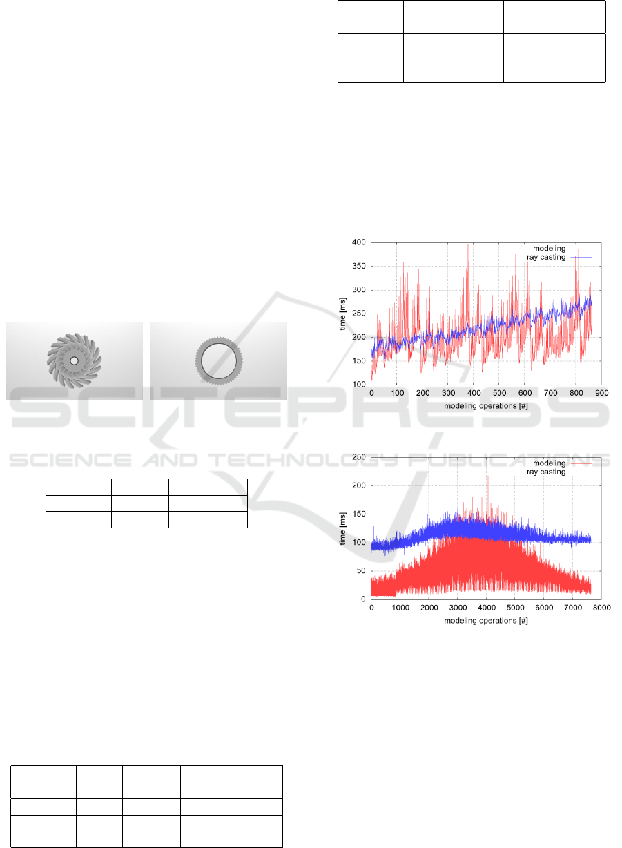
(a) Impeller (b) Gear

Figure 6: Resulting geometric objects.

Table 1: Point cloud size of initial and subtractive objects.

Example Initial Subtractive

Impeller 536959 19896

Gear 263854 44120

Table 2 and Table 3 summarize the measured

times in milliseconds for ﬁtting and rendering of one

frame. As the MPU and SLIM implementations do

not make use of parallel code exeuction, we pro-

vide single-threaded measurements (Our

ser

) in addi-

tion to multi-threaded ones (Our

par

). Given the non-

embarrassingly parallel nature of overall ﬁtting we

cannot achieve the theoretical maximum speedup, yet

still outperform the single threaded alternatives in all

but one test. Even if we switch to serial execution

our approach to rendering outperforms the alterna-

tives due to conceptual differences.

Table 2: Comparison of ﬁtting times in milliseconds.

Example MPU SLIM Our

ser

Our

par

Imp.

init

6300 107711 13684 1369

Imp.

sub

870 1720 2541 751

Gear

init

4339 51423 6870 1061

Gear

sub

2671 2158 9130 2925

Table 3: Comparison of rendering times in milliseconds.

Example MPU SLIM Our

ser

Our

par

Imp.

init

15930 1750 778 125

Imp.

sub

6548 510 394 112

Gear

init

16923 870 406 90

Gear

sub

26311 1570 1308 270

Benchmarking of Geometric Modeling Examples.

In both of these examples the simulation starts with

an initial geometry and consecutively applies set-

theoretic difference operations. The measured model-

ing times vary considerably depending on the amount

of cells affected by the respective operation. The

number of already completed modeling steps has only

negligible impact (see Figure 7).

(a) Impeller

(b) Gear

Figure 7: Measured times for modeling and visualization of

one frame.

Analyzing the rendering performance, one can see

that the number of already completed modeling oper-

ations only marginally impacts our visualization ap-

proach. Figure 6 presents the resulting geometric ob-

jects after the completion of all modeling operations

from the perspective used for the visualization bench-

marking. Even though modeling in example Impeller

affects large parts in image space and rendering times

are bound to rise, there is only moderate growth in

rendering time. In example Gear the rendering times

Efﬁcient Visualization and Set-theoretic Difference Operations for Accurate Geometric Modeling in Real-time Simulations

305

stay almost constant, because only very small parts in

image space are affected by the overall modeling.

7 CONCLUSIONS

The experimental results have proven that our ap-

proach is proper for precise geometric modeling in

real-time simulations. The number of already com-

pleted modeling operations has only a minor perfor-

mance impact on the algorithms processing the geo-

metric model, provided the surface elimination works

in an efﬁcient way. Currently the surface elimination

algorithm uses as smallest elimination granularity the

cells of the hierarchical modeling grid at the ﬁnest

level. A cell is marked for deletion, if it is completely

covered by a geometric modeling operand. A future

extension to the elimination strategy is the detection

of complete containment of one geometric operand in

another one on surface cell level, which is not limited

by ﬁxed spatial boundaries. Some additional points

for future improvements are:

• The visualization routine would beneﬁt from an

implementation for Graphics Processing Units

(GPUs), due to the embarrassingly parallel prob-

lem formulation of ray casting.

• Introduction of set theoretic union operation re-

quiring an extension to the surface elimination

and visualization strategy.

ACKNOWLEDGEMENTS

This project is co-ﬁnanced by the European Fund for

Regional Development (EFRE) and the state of Upper

Austria as part of the program “Investing in Growth

and Jobs” (IWB). Further information can be found

on https://www.iwb2020.at.

REFERENCES

Bastos, T. and Celes, W. (2008). Gpu-accelerated adap-

tively sampled distance ﬁelds. In 2008 IEEE Inter-

national Conference on Shape Modeling and Applica-

tions, pages 171–178.

Diener, C. L. (2012). Procedural modeling with signed dis-

tance functions. Unpublished bachelor’s thesis, Karl-

sruher Institute of Technology, Karlsruhe, Germany.

Frisken, S. F., Perry, R. N., Rockwood, A. P., and Jones,

T. R. (2000). Adaptively sampled distance ﬁelds: A

general representation of shape for computer graph-

ics. In Proceedings of the 27th Annual Conference on

Computer Graphics and Interactive Techniques, SIG-

GRAPH ’00, pages 249–254, New York, NY, USA.

ACM Press/Addison-Wesley Publishing Co.

Hart, J. C. (1996). Sphere tracing: a geometric method for

the antialiased ray tracing of implicit surfaces. The

Visual Computer, 12(10):527–545.

Kalojanov, J., Billeter, M., and Slusallek, P. (2011). Two-

level grids for ray tracing on gpus. Computer Graph-

ics Forum, 30(2):307–314.

Menon, J. (1996). An introduction to implicit techniques.

In Course Notes of the 23rd Annual Conference on

Computer Graphics and Interactive Techniques - Im-

plicit Surfaces for Geometric Modeling and Computer

Graphics, pages 13–26, New Orleans, LA, USA.

MPU (2003). Mpu software. http://home.eps.hw.ac.uk/

∼

ab226/software/mpu implicits/mpu/mpu oct 03.zip.

Retrieved July 7, 2016, from Heriot Watt University.

Museth, K. (2013). Vdb: High-resolution sparse vol-

umes with dynamic topology. ACM Trans. Graph.,

32(3):27:1–27:22.

Ohtake, Y., Belyaev, A., and Alexa, M. (2005). Sparse

low-degree implicit surfaces with applications to high

quality rendering, feature extraction, and smoothing.

In Proceedings of the Third Eurographics Sympo-

sium on Geometry Processing, SGP ’05, Aire-la-Ville,

Switzerland, Switzerland. Eurographics Association.

Ohtake, Y., Belyaev, A., Alexa, M., Alexa, M., Turk, G.,

and Seidel, H.-P. (2003). Multi-level partition of unity

implicits. ACM Trans. Graph., 22(3):463–470.

Roth, S. D. (1982). Ray casting for modeling solids. Com-

puter Graphics and Image Processing, 18(2):109 –

144.

SLIM (2005). Slim software. http://www.riken.go.jp/

lab-www/VCAD/VCAD-Team/members/ohtake/

slim/. Retrieved July 7, 2016, from RIKEN.

Wald, I., Ize, T., Kensler, A., Knoll, A., and Parker, S. G.

(2006). Ray tracing animated scenes using coherent

grid traversal. ACM Trans. Graph., 25(3):485–493.

Wald, I., Mark, W. R., G

unther, J., Boulos, S., Ize, T., Hunt,

W., Parker, S. G., and Shirley, P. (2009). State of the

art in ray tracing animated scenes. Computer Graphics

Forum, 28(6):1691–1722.

GRAPP 2020 - 15th International Conference on Computer Graphics Theory and Applications

306