
Algorithm for Extracting Initial and Terminal Contact Timings
during Treadmill Running using Inertial Sensors
Laura Prijot
1
, Cédric Schwartz
1
, Julien Watrin
2
, Alex Mendes
3
, Jean-Louis Croisier
1
,
Bénédicte Forthomme
1
, Vincent Denoël
1
, Olivier Brüls
1
and Mohamed Boutaayamou
1,4
1
Laboratory of Human Motion Analysis, University of Liège (ULiège), Liège, Belgium
2
ECAM Brussels Engineering School, Brussels, Belgium
3
Université de Reims Champagne-Ardenne, Reims, France
4
INTELSIG Laboratory, Department of Electrical Engineering and Computer Science, ULiège, Liège, Belgium
Keywords: Running, Gait, Algorithm, Concurrent Validation, Initial Contact, Terminal Contact, Temporal Events, Stride,
Stance, Swing, Gyroscope, Accelerometer, IMU.
Abstract: Inertial measurement units (IMUs) are now considered as an economical solution for long term assessment in
real conditions. However, their use in running gait analysis is relatively new and limited. Detecting the timing
at which the foot strikes the ground (initial contact, IC) and the timing at which the foot leaves the ground
(terminal contact, TC) gives access to many relevant temporal parameters such as stance, swing or stride
durations. In this paper, we present an original algorithm to extract IC and TC timings and associated
parameters from running data. These data have been measured using a newly developed IMU-based hardware
system in ten asymptotic participants who ran at three speeds (slow, normal, and fast) with different running
patterns (natural, rearfoot strike, mid-foot strike, and forefoot strike). This algorithm has been validated
against a 200 Hz video camera based on 7056 IC and TC timings and 6861 temporal parameters. This
algorithm extracted ICs and TCs with an accuracy and precision of (median [1
st
quartile; 3
rd
quartile]) 5 ms [-
5 ms, 15 ms] and 0 ms [-5 ms, 5 ms], respectively. The relative errors in the extraction of stride and stance
durations are -1.56 ± 3.00% and 0.00 ± 1.32%, respectively.
1 INTRODUCTION
Quantitative analysis of running is of critical interest to
the sports science field. For example, this analysis can
give insight into aetiology or treatment and recovery of
running injuries. In the same manner, it can help sports
coaches to improve the performances of their athletes.
Initial contact (IC) and terminal contact (TC) are key
timings in running: IC occurs at landing when the foot
initiates contact with the ground while TC is when the
foot ends contact. From these two key timings, it is
possible to compute relevant temporal parameters,
such as stance, swing or stride durations.
The stance phase, also known as the ground-
contact phase, starts at the foot IC and ends at TC. The
swing phase starts at TC and ends at the next IC.
Finally, a stride phase is the duration between two
ipsilateral ICs. Temporal parameters are related to
running performances: for instance, a shorter contact
time is linked to a good running economy and a faster
speed (Weyand, 2000).
Traditionally, timings are detected by using force
platforms. Nevertheless, these systems can only be
used in controlled laboratory environments where the
capture volume could be limited to a few steps.
The rapid technological advances in micro-electro-
mechanical systems have allowed the inertial
measurement units (IMUs) to become light, small, and
relatively cheap. Due to their portability and low power
consumption, IMU-based systems allow obtaining real
condition data.
IMUs have shown to give accurate and reliable
information on walking (Boutaayamou et al., 2015 and
2016). However, running differs from walking. As the
speed increases, the double support phase (both feet
simultaneously touching the ground) of the walking
gait cycle is replaced by a double swing phase, where
both feet are in the air. Indeed, by definition, someone
is running if both feet are never simultaneously
touching the ground. Moreover, when walking, people
are usually landing on their heel first. However, during
running, there are three possible different landing
strategies: rearfoot strike (RFS), mid-foot strike
258
Prijot, L., Schwartz, C., Watrin, J., Mendes, A., Croisier, J., Forthomme, B., Denoël, V., Brüls, O. and Boutaayamou, M.
Algorithm for Extracting Initial and Terminal Contact Timings during Treadmill Running using Inertial Sensors.
DOI: 10.5220/0008983402580265
In Proceedings of the 13th International Joint Conference on Biomedical Engineering Systems and Technologies (BIOSTEC 2020) - Volume 4: BIOSIGNALS, pages 258-265
ISBN: 978-989-758-398-8; ISSN: 2184-4305
Copyright
c
2022 by SCITEPRESS – Science and Technology Publications, Lda. All rights reserved

(MFS), and forefoot strike (FFS). Compared to
walking, the biomechanics involved in running is also
different: a wider range of motion of all the lower limb
joints, higher impact forces, and higher eccentric
muscle contraction (Nicola et al., 2012).
The use of IMU sensors in running gait analysis is
relatively new. In the literature, different localisations
for IMU sensors are considered such as trunk
(Bergamini et al., 2012) or tibia (Purcell et al., 2006).
Among all existing studies, only a few of them
include a concurrent validation of their algorithm
using a reference system. Both Chew et al. (2017) and
Falbriard et al. (2018) used the signal of an IMU
placed on the dorsal side of the foot to compute ICs
and TCs. The first one used a threshold-based
method, while the second one compared different
algorithms. However, to the authors’ knowledge,
there is no study available using foot-worn IMU
sensors that take into account the different existing
landing strategies.
In this work, we present a newly developed
algorithm to extract IC timing and TC timing
extracted from IMU signals measured at the level of
the foot (toe and heel). From these timings, the
ipsilateral stance, swing, and stride durations are
computed. This algorithm is tested on data obtained
from ten healthy participants running at steady speeds
on a treadmill. Furthermore, we validated this
algorithm against synchronously recorded reference
data obtained from a frame-by-frame analysis of 2D
high-speed (200 Hz) videos.
2 METHOD
2.1 Participants and Treadmill
Running Setting
In total, ten asymptotic participants (7 men and 3
women), who were regularly active at the time of the
tests, were volunteered for this study. The set of
participants includes both recreational and professional
runners. They were all informed with the procedure
and they have all signed an informed consent.
Table 1 shows the anthropometric characteristics
(mean ± standard deviation (STD)) of these
participants. Among them, seven were naturally RFS
while two were MFS, and one was FFS.
Each participant was equipped with an IMU-based
hardware system (Boutaayamou et al., 2019)
integrating three-axis accelerometers (range: ±16 g)
and three-axis gyroscopes (range: 2000 deg/s). This
system includes an acquisition box (memory, micro-
controller, and battery) linked by wires
to four small
Table 1: Anthropometric characteristics of the participants
measured at the time of the test.
Mean ± STD
A
g
e [
y
ears] 26.1 ± 3.9
Hei
g
ht [cm] 179.3 ± 11.4
Bod
y
mass [k
g
] 70.0 ± 12.3
IMU sensors (2.1 × 1.0 × 0.8 cm, weight = 16 g).
Consequently, it is portable with an autonomy of 4h30.
The IMU acquisition frequency is 200 Hz. No
restrictions on the shoes were imposed, to enlarge the
range of applications of the algorithm.
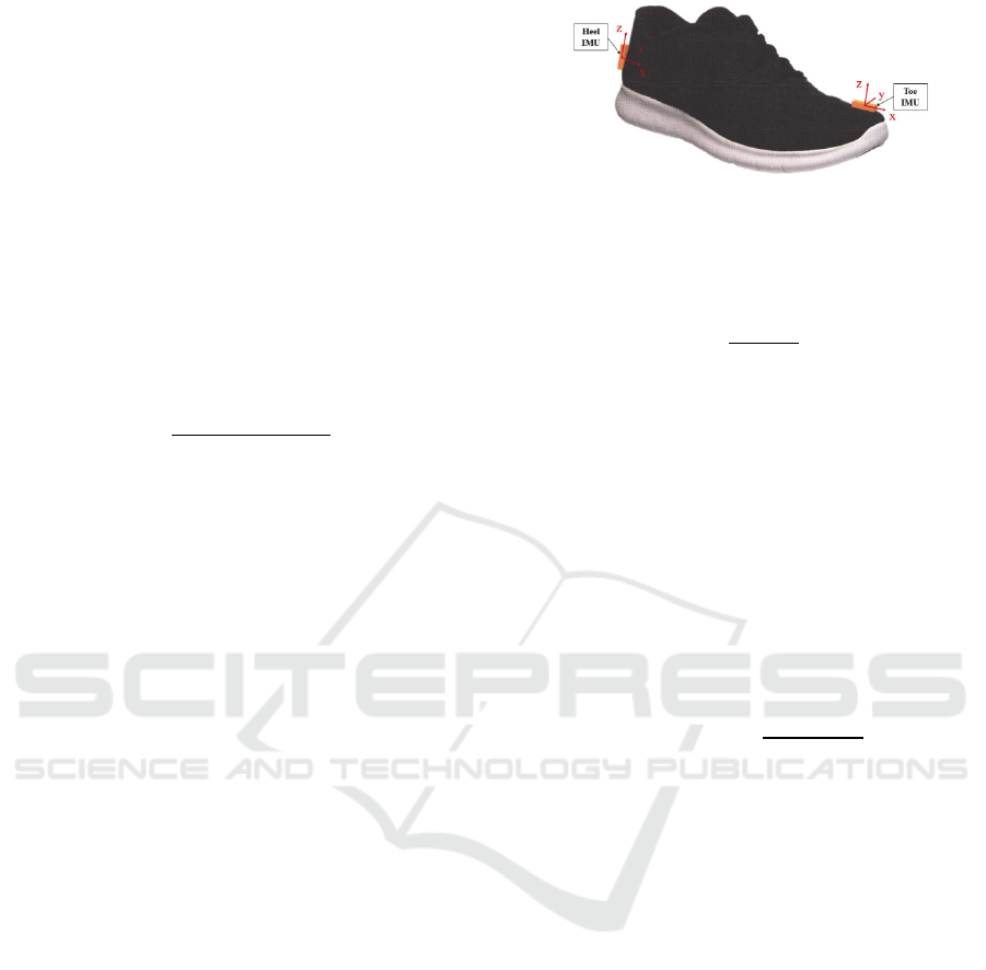
The sensors were directly attached to the right shoe
at the level of the first distal phalange (toe), calcaneus
(heel), the fifth metatarsal, and dorsal side of the foot.
In this work, only the toe and the heel sensors will be
considered. The fixation procedure used has been
validated in the case of walking (Boutaayamou et al.,
2015) and shows satisfying results for running gait
analysis.
The three-dimensional linear acceleration signals
[m/s
2
] are denoted by 𝑎
, 𝑎
, and 𝑎
, while the three-
dimensional angular velocity signals [deg/s] are
denoted by 𝜔
, 𝜔
, and 𝜔
along sensitive axes
represented schematically in Figure 1 .
Each test began with a standardized time to warm
up and to become familiar with the treadmill and
instrumentation system (during approximately five
minutes). At the same time, a preferential running
speed (PRS) is selected with the participant, at which
he should be able to run during ten minutes without
loss of intensity. The PRS (mean ± STD) of the
volunteers is 8.3 ± 1.3 km.h
−1
. During the tests, they
were asked to run at three different speeds: slow
(computed by PRS−0.25×PRS), normal (PRS), and
fast (computed by PRS+0.25×PRS). At each speed, the
participants performed six trials (in the following
order): three with a natural foot strike pattern, one
rearfoot strike (RFS), one mid-foot strike (MFS), and
one forefoot strike (FFS). In total, the participants were
asked to perform 18 trials of 60 s. The minimum total
test duration was 69 minutes per participant, including
3 minutes of rest between each trial. All running tests
were performed at the Laboratory of Human Motion
Analysis (University of Liège, Belgium), on a
treadmill (SportsArt T650). At the same time, all the
trials were recorded using a 2D high-speed video
camera (Basler Pilot) with a sampling frequency of 200
Hz. This video camera will be used as the reference
system. Signal and data processing were carried out
using the software Matlab
®
(R2017a, Mathworks,
Natick, MA, USA).
Algorithm for Extracting Initial and Terminal Contact Timings during Treadmill Running using Inertial Sensors
259
2.2 Extraction Algorithm of IC and TC
Timings
The proposed algorithm first computes an estimated
IC based on the average stride duration. Then, an
exact IC timing is obtained from the different linear
accelerations. Subsequently, TCs are found between
two successive ICs.
The first step is to obtain an estimated average
stride duration, 𝑑
[
𝑠
]
, based on the Fourier Fast
Transform of the heel angular velocity signal (heel
𝜔
). The first peak, which is also the highest,
corresponds to the stride frequency [Hz]. 𝑑
is,
then, obtained from this stride frequency using the
following formula
𝑑
=
1
stride frequenc
y
.
(1)
Alternatively, 𝑑
can be obtained from the
auto-correlation of the same signal. In that case, the
positive lag corresponding to the first positive local
maxima after 0 is the average 𝑑
(available in
Matlab
®
using the function xcorr).
After computing 𝑑
, estimated ICs are
obtained in the filtered heel 𝜔
signal. The filter used
is a high pass Butterworth filter of order 4 with a cut-
off frequency of 15 Hz. A high pass filter allows to
remove the movement components of the signal and
to keep only the shock parts. Estimated ICs can then
be obtained by detecting a minimum in the filtered
heel 𝜔
. The distance between two successive
minima is imposed to be of at least 85% of 𝑑
,
allowing for small variations of 𝑑
at each stride.
Potential exact ICs are obtained by looking for
local extrema, in a time window around the estimated
IC, in different linear acceleration signals of both
sensors. Namely, the algorithm is looking for: a local
minimum in toe 𝑎
, local minimum in toe 𝑎
, local
minimum in heel 𝑎
, and local maximum in heel 𝑎
,
in the time window [-20 ms; 5 ms] around the
estimated IC.
Then, the exact IC corresponds to the first time
instant among all these extrema. The acceleration
signals in the transverse direction (Y-axis) are not
considered
since they are runner dependent. For
instance, they can be influenced by foot movements
like supination or pronation.
As the tip is always the last part of the foot in
contact with the treadmill, TCs will be detected using
the toe sensor. The toe total acceleration in the sagittal
plane, given by has shown the highest accuracy.
Figure 1: Schematic illustration of the position of the IMU
sensors used in the proposed algorithm, including the three
local axes (X-axis, Y-axis, and Z-axis). The two sensors are
placed on the right shoe at the level of the first distal phalange
(toe) and at the calcaneus (heel).
𝑎
=
𝑎
+𝑎
,
(2
)
TCs are determined based on the intuitive
principle that there is always a TC between two
successive ICs. Hence, for each stride i, a TC(i) will
be searched in the time window between IC(i) and
IC(i+1). This window can be further reduced to
increase the accuracy of the event extraction method.
The upper bound of the time interval can be obtained
based on the definition of running: someone is
running if there is a double float phase, where both
legs are in the swing phase simultaneously. This is
only possible if the stance phase lasts for less than
50% of the stride duration.
Hence, the upper limit is defined as follows
𝐿𝑖𝑚
=𝐼𝐶
(
𝑖
)
+
(
)
()
.
(3)
This limits the application of the algorithm to only
running cases. However, this improves the accuracy.
In fact, in some cases, the acceleration linked to the
swing movement of the foot is higher than the shock
corresponding to the TC (see Figure 2).
Furthermore, the lower bound of the time window
(𝐿𝑖𝑚
) is obtained using the entropy of the signal.
During the stance phase, the foot has a constant
acceleration and this signal flat zone is characterized
by a low entropy. Hence, the lower limit is obtained
by computing the entropy over a sliding window. The
size of the window has been determined empirically:
on one side, it should be as small as possible to have
good local information. On the other side, it
must be
large enough to not detect the flatter zone that
appears for some runners after the toe-off peak.
This was generally a problem for FFS running
patterns. A window of 15 samples (i.e., 75 ms) has
shown good results for all participants.
𝑇𝐶(𝑖) is then determined by finding a maximum
in the toe sagittal acceleration signal over the time
window : [𝐿𝑖𝑚
(
𝑖
)
; 𝐿𝑖𝑚
(𝑖)].
BIOSIGNALS 2020 - 13th International Conference on Bio-inspired Systems and Signal Processing
260
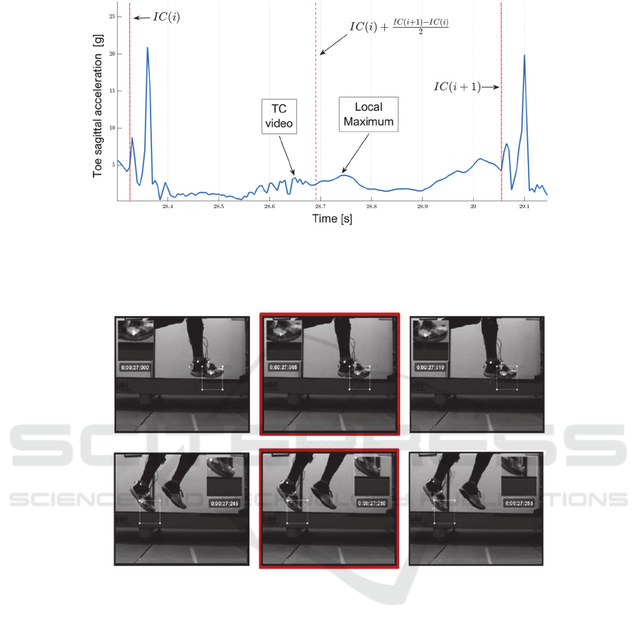
Figure 2: Determination of TCs using the toe sagittal acceleration signal. TC is found between two successive ICs. An upper
limit can be obtained using the definition of running: the stance duration must be less than 50% of the stride duration. This
prevents to wrongly detect local maximum coming from the movement acceleration. The signal flat phase can be used as a lower
limit, which can be detected using the entropy of the signal over a sliding window.
Figure 3: Determination of IC and TC timings using the 2D high-speed video camera. IC (upper pictures) is the first frame
where the pixels representing one shoe are directly in contact with those representing the belt of the treadmill. TC (lower
pictures) corresponds to the last frame where the pixels of the shoe are in contact with those of the treadmill.
2.3 Concurrent Validation and
Evaluation Methods
The reference timings are obtained from a frame-by-
frame analysis of 2D high speed videos. A precise
definition is used to select the frame corresponding to
an IC and to a TC: IC is the first frame where the pixels
representing one shoe are directly in contact with those
representing the belt of the treadmill. In other words, it
is the first frame where there are no white pixel (i.e.,
background pixel) in-between the shoe and the
treadmill.
Conversely, TC corresponds to the last frame
where the pixels of the shoe are in contact with those
of the treadmill (see Figure 3).
Finally, the different temporal parameters are
computed from IC and TC timings, as follows
𝑑
(
𝑖
)
=𝑇𝐶
(
𝑖
)
𝐼𝐶
(
𝑖
)
,
(4
)
𝑑
(
𝑖
)
=𝐼𝐶
(
𝑖+1
)
𝑇𝐶
(
𝑖
)
,
(5
)
𝑑
(
𝑖
)
=𝐼𝐶
(
𝑖+1
)
𝐼𝐶(𝑖).
(6
)
The reference system has a maximum achievable
resolution of 5 ms. Additionally, at some point in the
video, there are two identical frames following each
other. In that case, a 5 ms error can also occur.
These reference timings are used to concurrently
validate the events obtained using the proposed
algorithm. For each stride, the results for (1) IC, (2) TC,
Algorithm for Extracting Initial and Terminal Contact Timings during Treadmill Running using Inertial Sensors
261

(3) 𝑑
, and (4) 𝑑
are computed. The results
for 𝑑
have been computed but are not shown in
this paper
Finally, the accuracy and precision of ICs and TCs
extraction is quantified by the mean and STD or
median and inter-quartile range (IQR) values (i.e., 1
st
quartile (Q
1
); 3
rd
quartile (Q
3
)) of the differences
between these timings and the reference system,
depending on the normality of data distributions. This
is done for each participant separately and for all
participants together. The normality of data
distributions is tested using Jarque-Bera test (available
in Matlab
®
using the function jbtest). Additionally,
relative errors are computed as the mean of the stride-
by-stride differences between the IMU temporal
parameter and the reference temporal parameter
divided by the reference temporal parameter. These
errors are only meaningful for temporal parameters and
they will not be computed for timings.
3 RESULTS
This work focuses on running trials from the acquired
data. In some trials, particularly at low speeds, some
participants exhibited a double support phase.
Consequently, as these trials are considered as
walking trials, they have been excluded from this study.
In total, 39 trials out of 183 were not considered.
Additionally, some trials have been reclassified
according to the real running pattern observed that, in
some cases, was different from the supposed running
pattern. Indeed, some participants had difficulties in
voluntarily performing MFS or FFS.
First of all, an intra-participant comparison
between the IMU results and reference results is
carried out. In this paper, the median is used as the
data are not normality distributed. However, in
general in this study, the mean and median values and
STD values IQR ones were similar. The same
conclusion can be drawn for STD values IQR ones.
Table 2 summarizes the results for each
participant, the values have been rounded to the
sample period (i.e., 5 ms) of the hardware systems.
This analysis includes all the valid trials (different
speeds and different foot strikes) and at least 30 valid
strides per trial, when available. The number of
observations depends on the number of valid events
taken into account. In the case of ICs, the mean of the
extraction accuracies is 5 ms. Consequently, the
algorithm tends to detect the ICs one frame later than
the reference system. The mean of the extraction
precisions obtained in the case of IC is 10 ms.
Table 2: Intra-participant differences between IMU
timings/temporal parameters and reference data. It includes
the median and the interquartile range values ([1
st
quartile
Q
1
; 3
rd
quartile Q
3
]) as well as the number of observations
(nbr. of obs.).
Partici-
pants
Running
timings/
p
arameters
Median
[Q
1
; Q
3
]
[ms]
Nbr.
of obs.
1
IC
TC
𝑑
𝑑
0 [-10; 10]
0 [-5; 5]
5 [-5; 15]
0 [-10; 10]
211
205
205
191
2
IC
TC
𝑑
𝑑
-10 [-20; 0]
0 [-5; 5]
10 [-5; 25]
0 [-10; 10]
306
306
306
291
3
IC
TC
𝑑
𝑑
0 [-20; 20]
0 [-5; 5]
5 [-15; 25]
0 [-10; 10]
437
437
437
403
4
IC
TC
𝑑
𝑑
5 [0; 10]
0 [0; 10]
-5 [-10; 0]
0 [-10; 10]
366
366
365
348
5
IC
TC
𝑑
𝑑
10 [5; 15]
0 [-5; 5]
-10 [-15; -5]
0 [-10; 10]
484
394
385
462
6
IC
TC
𝑑
𝑑
10 [5; 15]
0 [-5; 5]
-10 [-15; -5]
0 [-5; 5]
332
332
332
314
7
IC
TC
𝑑
𝑑
15 [5; 25]
0 [-5; 5]
-15 [-30; 0]
0 [-10; 10]
129
129
129
125
8
IC
TC
𝑑
𝑑
0 [-15; 15]
0 [-5; 5]
0 [-20; 20]
0 [-15; 15]
312
213
213
303
9
IC
TC
𝑑
𝑑
10 [5; 15]
0 [-5; 5]
-5 [-15; 5]
0 [-10; 10]
468
450
448
451
10
IC
TC
𝑑
𝑑
5 [-15; 25]
0 [-5; 5]
-5 [-25; 15]
0 [-10; 10]
608
571
567
586
The worst-case for the IC determination appears for
participants 3 and 10, with an IQR of 20 ms away
from the median value. The best case is for participant
4 with a median error of one sample (i.e., 5 ms) and
IQR of 5 ms around this median error. In that case,
the precision obtained exactly corresponds to the
maximum achievable precision. Indeed, the
maximum precision depends on the sampling rate of
BIOSIGNALS 2020 - 13th International Conference on Bio-inspired Systems and Signal Processing
262

both the IMU system and the high-speed video, as
well as the 5 ms error than can be explained by errors
in the reference system.
In the case of TCs, the results obtained with IMU
are similar to those obtained with the reference
system. Indeed, the mean of median errors between
the two systems is 0 ms and the mean of the IQRs is
5 ms, for all participants. Therefore, the algorithm can
detect TCs with the maximum possible accuracy.
For the stance duration, the algorithm tends to
underestimate the duration compared to the reference
values. This can be explained by the fact that ICs are
generally detected later with the algorithm. The mean
of the median values is -3 ms, which is less than one
sample of difference and less than the maximum
accuracy. The mean of the variability values is 12.5 ms,
this is slightly higher than the maximum precision
expected. Indeed, IC(i) can be determined with a
maximum precision of 5 ms and TC(i) can also be
determined with a maximum precision of 5 ms. As the
errors may cumulate, a maximum precision of 10 ms is
expected for durations. However, the variability is of 5
ms for three participants out of ten.
Table 3: Inter-participant comparison including the
extraction accuracies and precisions of 7 participants,
running with their preferential running style at speeds
ranging from 7.1 to 9 km.h
-1
.
Running
timings/
parameters
Mean ±
STD
[ms]
Median
[Q
1
; Q
3
]
[ms]
Median
[Q
1
; Q
3
]
[%]
IC 5 ± 9 5 [-5; 15] /
TC 1 ± 4 0 [-5; 5] /
𝑑
-5 ± 15 -5 [-15; 5]
-1.56
[-4.56; 2.56]
𝑑
0 ± 10 0 [-10;10]
0.00
[-1.32; 1.32]
The accuracy for the stride duration is 0 ms for all
participants, which is the best possible achievable
accuracy. The precision obtained is on average 10 ms,
which is the expected precision, as explained before.
Note that, one participant out of the ten has a better
precision (5 ms) and only one participant has a worst
precision (15 ms) than the one expected.
Finally, an inter-participant comparison is done,
including only the natural foot strike trials at PRS
condition (i.e., three trials per participant). We did not
include the trials performed by three participants as at
least one of the three above mentioned trials was not
valid. The speed of the trials considered was between
7.1 and 9.0 km.h
-1
.
Table 3 provides the mean ± STD as well as the
median and IQR values of the differences between the
extracted IMU values and the reference values. The
mean errors and the median errors are similar for all
timings and temporal parameters. The extraction
precisions expressed in terms of STD are identical to
those expressed in terms of IQR except for the stance
duration, where the STD value is influenced by some
outlier values.
The extraction accuracy in the case of ICs is 5 ms.
The algorithm tends, then, to detected ICs one sample
later than those extracted by the reference system. This
could be explained by the fact that IMUs will detect the
interaction (shock) between the shoe and the belt of the
treadmill while, in the video, the selected frame is the
one when the shoe and the treadmill touch each other
but have not yet interacted. The precision obtained for
the ICs is 10 ms, which is one frame higher than the
maximum achievable precision. On the other side, TCs
are extracted with both the maximum achievable
accuracy (i.e., 0 ms) and precision (i.e., 5 ms).
The stance durations tend to be underestimated by
the algorithm. On average, they are 5 ms shorter than
those obtained with the reference system. Again, this is
explained by the fact that ICs have a tendency to be
detected 5 ms later with the IMUs. Finally, the stride
duration, which only depends on successive ICs, are
extracted with the best possible accuracy (i.e., 0 ms)
and a precision equal to the maximum expected
precision due to the accumulation of errors. Indeed,
there could be 5 ms of error in the first IC (IC(i)) and 5
ms of error for the successive IC (IC(i+1)). All in all,
it can be seen that the inter-participants and intra-
participant comparison give similar results.
It is also interesting to express the errors in both
stance and stride duration estimates as a percentage of
the total duration. The 𝑑
relative error is (median
[Q
1
, Q
3
]) -1.56 % [-4.56 %; 2.56 %] and the maximum
relative error is -9.52 %. The 𝑑
relative error is
(median [Q
1
, Q
3
]): 0.00 % [-1.32 %; 1.32 %] and the
maximum computed error is 4.49%.
4 DISCUSSION
This article presents an original algorithm to extract
the two main timings (ICs and TCs) at different
running speeds (slow, normal, and fast) and with
different running styles (natural, RFS, MFS, and
FFS). The data collected for this work are obtained
using two IMU sensors placed on regular shoes at the
level of the heel (calcaneus) and toe (first distal
phalange).
Algorithm for Extracting Initial and Terminal Contact Timings during Treadmill Running using Inertial Sensors
263

Only the right shoe has been used in this work.
However, the algorithm is supposed to work in the
same way for the left foot. Additionally, the IMU
hardware system used here can record the data of up
to four sensors at the same time. It is thus possible to
record the data of both legs simultaneously.
Therefore, it would be possible to obtain other
parameters, such as the step duration. Besides, it would
be possible to make a comparison between the two
legs, which has a wide range of applications, including
monitoring recovery after injury or surgery.
The performance of the algorithm is determined
by a concurrent validation with 2D high-speed
videos, recorded simultaneously. The algorithm
presented here has been concurrently validated using
a total of 7056 timings and 6861 temporal parameters.
This comparison has shown a good agreement
between timings obtained using the IMU signals and
timings detected on the 2D videos. The measures
include running speeds ranging from 6.0 to 11.3 km.h
-
1
. The obtained global extraction accuracy and
precision (median [Q
1
; Q
3
]) is 5 ms [-5 ms; 15 ms] and
0 ms [-5 ms; 5 ms] for, respectively, ICs and TCs.
Besides, the accuracy and precision for the stance
durations and stride durations (median [Q
1
; Q
3
]) are -5
ms [-15 ms; 5 ms] and 0 ms [-10 ms; 10 ms],
respectively. This corresponds to a relative error of
respectively -1.56 ± 3.00% and 0.00 ± 1.32%.
The stride duration average error obtained here
(i.e., 0 ms) is consistent with the one measured by
Chew et al. (2018), which is between -0.44 ms and
0.33 ms. However, Chew et al. (2018) used an
algorithm based on a thresholding-method that relies
on experimental values needed to determine the
threshold. This is not the case for the algorithm
presented here. Similarly, the stance duration errors
are similar to those found by Purcell et al. (2006).
They found an error (mean ± STD) of 0 ± 12 ms and
−2 ± 3 ms, depending on the running speed, using a
tibial accelerometer. However, they used a force
platform with higher accuracy than the 2D video
system used here. Falbriard et al. (2018) found better
accuracy and precision (median [Q
1
, Q
3
]): 2 [1 ms, 3
ms]
for IC and only a better precision for TC (4 ms [2
ms, 6 ms]). Nevertheless, this precision cannot be
achieved here with the 200 Hz reference system used.
The algorithm presented here is only valid for
steady state running over a treadmill. Walking cases
cannot be analysed using the present method,
however, there exist algorithms to detect the type of
activity (walking, running, and rest). Once the
activity is appropriately determined, either a walking
or a running algorithm can be selected to extract
temporal events.
5 CONCLUSION
In this article, we presented an original algorithm to
extract timings (IC and TC) in the case of steady-state
running over a treadmill, using IMU sensors. From
these two timings, three temporal parameters can also
be computed: stance, swing, and stride durations. The
method developed here has the following advantages:
- The sensors are placed on the shoes and not
directly on the feet, which allows running in
many different conditions.
- The algorithm only uses two IMU sensors per
foot: one at the level of the heel and the other at
the level of the first distal phalange (toe).
Additionally, only one sensor (i.e., toe sensor) is
used to determine TCs with the maximum
achievable precision and accuracy.
- This method has been concurrently validated
using a 2D high-speed video camera as the
reference system.
- The analysis is done over a large number of
strikes including a wide range of running speeds
(from 6 km.h
-1
to 11.3 km.h
-1
) and different
running styles (natural, RFS, MFS, and FFS).
The results showed that it is possible to achieve
acceptable accuracy and precision using a foot-worn
IMU-based system. These results are encouraging for
the use of IMU for daily and out-of-lab monitoring.
They can be seen as a good trade-off between
expensive and laboratory-limited measurement
instruments like force platforms that show high
accuracy and wearable systems that can be found in
smartwatches or in smartphones.
Future researches may focus on the use of a single
IMU sensor to extract the timings and associated
temporal parameters or on the detection of spatial
parameters like the stride length. Further work could
also focus on extracting the durations of the stride
sub-phases.
ACKNOWLEDGEMENTS
The authors would like to thank all the participants who
were volunteers for this study. We would also like to
thank the reviewers for their relevant comments, which
will be taken into consideration in future articles.
BIOSIGNALS 2020 - 13th International Conference on Bio-inspired Systems and Signal Processing
264

REFERENCES
Amini, N., Vahdatpour, A., Wenyao Xu, and Sarrafzadeh.,
M., 2011. Accelerometer-based on-body sensor
localization for health and medical monitoring
applications. Pervasive Mobile Computing, 7:746–760
Bergamini, E., Picerno, P., Pillet, H., Natta, F., Thoreux, P.,
and Camomilla, V., 2012. Estimation of temporal
parameters during sprint running using a trunk-
mounted inertial measurement unit. Journal of
Biomechanics, 45:1123–1126.
Benson, L., Clermont, C., Bošnjak, E., and Ferber, R., 2018.
The use of wearable devices for walking and running
gait analysis outside of the lab: A systematic review.
Gait & Posture, 63.
Boutaayamou, M., Denoël, V., Brüls, O.,Demonceau, M.,
Maquet, D., Forthomme, B., Croisier, J.-L., Schwartz,
C., Verly, J., and Garraux. G., 2016. Extraction of
temporal gait parameters using a reduced number of
wearable accelerometers.
Boutaayamou, M., Denoël, V., Brüls, O., Maquet, D.,
Forthomme, B., Croisier, J.-L., Schwartz, C., Verly, J.,
Macq, B., Garraux, G., and Stamatakis, J., 2015.
Development and validation of an accelerometer-based
method for quantifying gait events. Medical
Engineering and Physics, 37:226–232
Boutaayamou, M., Schwartz, C., Joris, L., Forthomme, B.,
Denoël, V., Croisier, J.-L., Verly, J. & Garraux, G., and
Brüls, O., 2019. Adaptive Method for Detecting Zero-
Velocity Regions to Quantify Stride-to-Stride Spatial
Gait Parameters using Inertial Sensors. 12th
International Conference on Bio-inspired Systems and
Signal Processing, 229-236.
Chew, D.-K., Ngoh, K., Gouwanda, D., and Gopalai., A.,
2017. Estimating running spatial and temporal
parameters using an inertial sensor. Sports
Engineering, 21(2):115–122.
Falbriard, F., Meyer, B., Mariani, G., Millet, P., and
Aminian, K., 2018. Accurate estimation of running
temporal parameters using foot-worn inertial sensors.
Frontiers in Physiology.
Hanley, B., Bissas, A., and Drake, A., 2015. The
contribution of the flight phase in elite race walking.
33rd International Conference on Biomechanics in
Sports, At Poitiers, France
Koska, D., Gaudel, J., Hein, T., and Maiwald, C., 2018.
Validation of an inertial measurement unit for the
quantification of rearfoot kinematics during running.
Gait & Posture, 64:135–140.
Maiwald, C., Sterzing, T., Mayer, T.A., and Milani, T.L.,
2009. Detecting foot-to-ground contact from kinematic
data in running. Footwear Science, 1(2):111–118.
Mariani, B., Rouhani, H., Crevoisier, X., and Aminian, K.,
2013. Quantitative estimation of foot-flat and stance
phase of gait using foot-worn inertial sensors. Gait and
Posture, 37(2):229 – 234.
Nicola, T. and Jewison, D., 2012. The anatomy and
biomechanics of running. Clinics in Sports Medicine,
31:187-201.
Nicolai, L., Mifsud, N., Kristensen, H., Villumsen, M.,
Hansen, J., and Kersting, U., 2014. Portable inertial
motion unit for continuous assessment of in-shoe foot
movement. Procedia Engineering, 72:208–213.
Purcell, B., Channells, J., James, D., and Barrett, R., 2006
Use of accelerometers for detecting foot-ground
contact time during running. Proc. SPIE
Weyand, P.G., Sternlight,, D. B., Bellizzi, M. J., and
Wright, S., 2000. Faster top running speeds are
achieved with greater ground forces not more rapid leg
movements. Journal of Applied Physiology,
89(5):1991–1999.
Wixted, A., Thiel, D., Hahn, A., Gore, C., Pyne, D., and
James, D., 2007. Measurement of energy expenditure in
elite athletes using mems-based triaxial
accelerometers. Sensors Journal, IEEE, 7:481–488.
Yang, S., Mohr, C., and Li, Q., 2011. Ambulatory running
speed estimation using an inertial sensor. Gait and
Posture, 34(4):462 – 466.
Algorithm for Extracting Initial and Terminal Contact Timings during Treadmill Running using Inertial Sensors
265
