
A Fast Algorithm for Unsupervised Feature Value Selection
Kilho Shin
1
, Kenta Okumoto
2
, David Lowrence Shepard
3
, Tetsuji Kuboyama
1
, Takako Hashimoto
4
and Hiroaki Ohshima
5
1
Gakushuin University, Tokyo, Japan
2
Japan Post Bank, Tokyo, Japan
3
UCLA, Scholary Innovation Lab., CA, U.S.A.
4
Chiba University of Commerce, Chiba, Japan
5
University of Hyogo, Kobe, Japan
takako@cuc.ac.jp, ohshima@ai.u-hyogo.ac.jp
Keywords:
Unsupervised Learning, Feature Selection.
Abstract:
The difficulty of unsupervised feature selection results from the fact that many local solutions can exist simul-
taneously in the same dataset. No objective measure exists for judging the appropriateness of a particular local
solution, because every local solution may reflect some meaningful but different interpretation of the dataset.
On the other hand, known accurate feature selection algorithms perform slowly, which limits the number of
local solutions that can be obtained using these algorithms. They have a small chance of producing a feature
set that can explain the phenomenon being studied. This paper presents a new method for searching many
local solutions using a significantly fast and accurate algorithm. In fact, our feature value selection algorithm
(UFVS) requires only a few tens of milliseconds for datasets with thousands of features and instances, and
includes a parameter that can change the local solutions to select. It changes the scale of the problem, allowing
a user to try many different solutions and pick the best one. In experiments with labeled datasets, UFVS found
feature value sets that explain the labels, and also, with different parameter values, it detected relationships
between feature value sets that did not line up with the given labels.
1 INTRODUCTION
Feature selection has been an area of considerable re-
search in machine learning. In the era of big data,
feature selection algorithms must be both highly effi-
cient with large, complex datasets and independent of
class labels.
In addition, data found in the cloud often includes
more categorical values and numerical values than
traditional statistical data. Categorical data can eas-
ily be converted into numeric data and vice-versa:
one-hot encoding is a common algorithm for convert-
ing categorical values into vectors of numerical val-
ues. Many discretization algorithms are known for the
conversion of numerical values into categorical (dis-
crete) values. In this paper, we focus on feature selec-
tion for categorical data and assume that numerical
values in datasets have been appropriately discretized
beforehand. Hence, we assume that all features in
each dataset take only a finite number of categori-
cal values. Feature selection on categorical data in
supervised learning has been studied intensively. In
supervised learning, feature selection is a process for
finding a subset of the features of a dataset that max-
imizes the relevance, or correlation, of the subset to
class labels. In fact, Almualllim et al. (Almuallim
and Dietterich, 1994) propose an algorithm that per-
forms a breadth first search of the Hasse diagram of an
entire feature set. Almuallim’s algorithm starts from
the empty set node and stops when it reaches a fea-
ture set whose Bayesian risk vanishes. Bayesian risk
is used as a measure of correlation of feature set to
class labels: the smaller the Bayesian risk of a feature
set is, the more relevant the set is to class labels. How-
ever, this algorithm is inefficient with a large number
of features because the size of a Hasse diagram in-
creases exponentially with the number of features.
On the other hand, Hall (Hall, 2000) and Peng
et al. (Peng et al., 2005) propose a view of fea-
ture selection as a process for building a set of rele-
vant features without redundancy. A relevant feature
is a feature highly correlated to class labels, while
Shin, K., Okumoto, K., Shepard, D., Kuboyama, T., Hashimoto, T. and Ohshima, H.
A Fast Algorithm for Unsupervised Feature Value Selection.
DOI: 10.5220/0008981702030213
In Proceedings of the 12th International Conference on Agents and Artificial Intelligence (ICAART 2020) - Volume 2, pages 203-213
ISBN: 978-989-758-395-7; ISSN: 2184-433X
Copyright
c
2022 by SCITEPRESS – Science and Technology Publications, Lda. All rights reserved
203
a redundant feature in a feature set has strong cor-
relation with other features in the same set. Ac-
cording to Battiti’s recommendation (Battiti, 1994),
the correlation is measured using mutual information.
In fact, Maximum-Relevance-Minimum-Redundancy
(mRMR) (Peng et al., 2005) is a forward-selection al-
gorithm and iterates selection of a feature that shows
the best balance between mutual information to class
labels (relevance) and a sum of mutual information to
the features selected so far (redundancy). This greedy
algorithm has improved the efficiency of the feature
selection algorithms known so far, partly because it
avoids evaluation of correlation for feature sets: the
number of pairs of distinct features is n(n − 1)/2,
while the number of feature subsets is determined by
2
n
.
One problem with this approach is that it does not
incorporate interaction among features into the deter-
mination of relevance. Two or more features are said
to mutually interact when each individual feature has
no strong correlation to class labels but all the fea-
tures together strongly correlate to class label. Zhao et
al. (Zhao and Liu, 2007a) propose a practically fast al-
gorithm that incorporates such interaction into the re-
sults of selection, while Shin et al. (Shin et al., 2017)
further improved the efficiency and propose signifi-
cantly fast algorithms that can scale to real big data.
Study of unsupervised feature selection is, on the
other hand, more challenging, because class labels
cannot be used to guide selection. As a substitute
for class labels, pseudo-labels generated by cluster-
ing can be used to convert unsupervised problems
into supervised problems (Qian and Zhai, 2013; LI
et al., 2014; Liu et al., 2016). Also, some stud-
ies use preservation of manifold structures (He et al.,
2005; Cai et al., 2010; Zhao and Liu, 2007b) and
data-specific structures (Wei et al., 2016; Wei et al.,
2017) as criteria of selection. In many cases, however,
computationally-intensive procedures such as matrix
decomposition are used to solve optimization prob-
lems. More importantly, the proposed algorithms aim
to find a single answer which is merely a local so-
lution. Since pseudo-labels and structures are derived
from the entire feature set, which can include data that
should be understood as noise or outliers for the pur-
pose of selection, the solution can be inappropriate.
In contrast, this paper aims to develop a signifi-
cantly fast algorithm for unsupervised feature selec-
tion that is equipped with an adjustable parameter to
change local solutions that the algorithm selects. By
leveraging these attributes of the algorithm, we can
test a number of different parameter values. As a re-
sult, we can choose better solutions from the pool of
solutions that the algorithm finds.
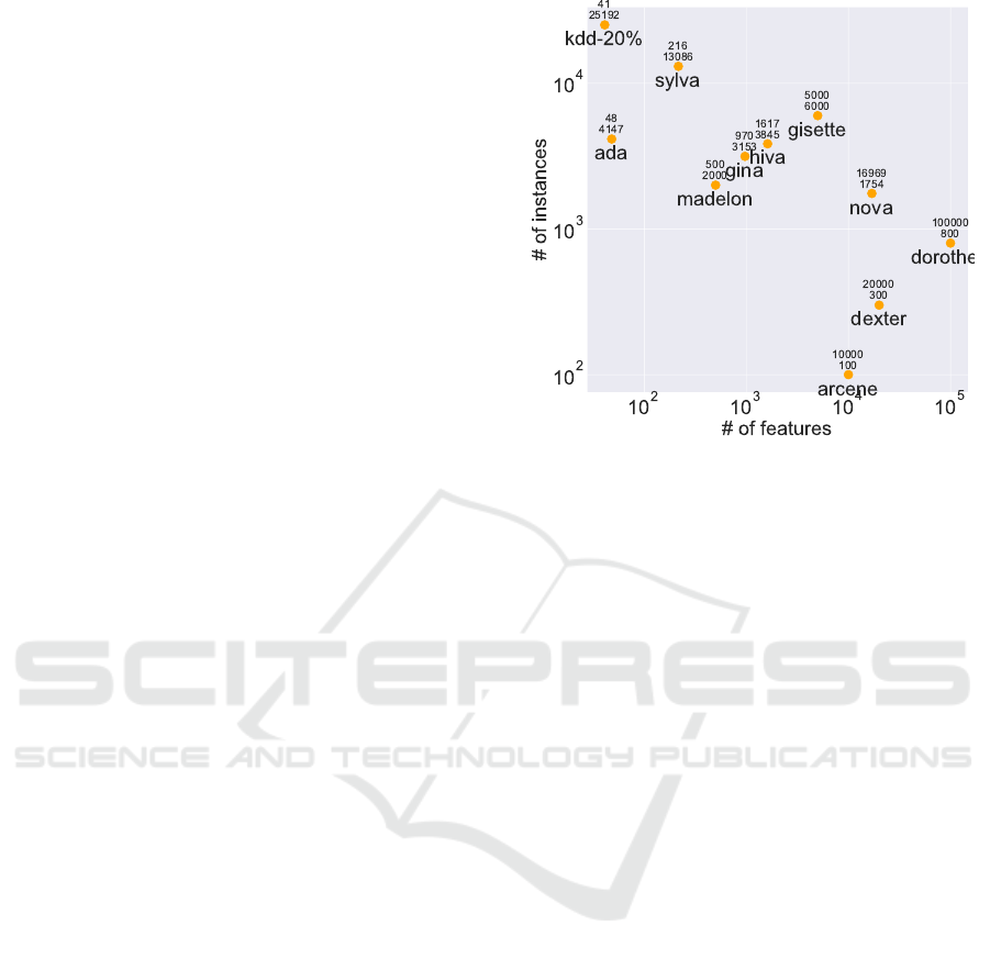
Figure 1: Eleven datasets used in our experiment.
2 PRELIMINARY ASSUMPTIONS
AND NOTATIONS
In this paper, we assume that all continuous values
specified in a dataset are discretized beforehand, and
a feature always takes a finite number of categorical
values.
For the purpose of analysis, we use 11 relatively
large datasets of various types taken from the litera-
ture (Fig. 1): five from NIPS 2003 Feature Selection
Challenge, five from WCCI 2006 Performance Pre-
diction Challenge, and one from KDD-Cup. For con-
tinuous features included in the datasets, we catego-
rize the values of such features into five equally long
intervals before using them. The instances of all of
the datasets are annotated with binary labels.
In this paper, a dataset D is a set of instances and
F denotes the entire set of the features that describe
D. A feature f ∈ F is a function f : D → R( f ), where
R( f ) denotes the range of f , which is a finite set
of values. Also, we often treat f as a random vari-
able with the empirical probability distribution de-
rived from the dataset. That is, when N( f = v) de-
notes the number of instances in a dataset D that have
the value v at the feature f , Pr( f = v) = N( f = v)/|D|
determines the empirical probability.
A feature set S ⊆ F can be viewed as a random
variable associated with the joint probability for the
features that belong to S: for a value vector v
v
v =
(v
1
,...,v
n
) ∈ R( f
1
)×···×R( f
n
), Pr(S = v
v
v) = N( f
1
=
v
1
,..., f
n
= v
n
)/|D| determines the joint probability
for S = { f
1
,..., f
n
}. Furthermore, we introduce a ran-
dom variable C to represent class labels of instances,
ICAART 2020 - 12th International Conference on Agents and Artificial Intelligence
204

when the dataset is labeled.
Our method uses several measures from informa-
tion theory defined for the random variables X and Y .
The entropy of X is determined and denoted by
H(X) = −
∑
x
Pr(X = x)log
2
Pr(X = x), (1)
and mutual information (MI) between X and Y is
given by
I(X ;Y ) =
∑
x
∑
y
Pr(X = x,Y = y)·
log
2
Pr(X = x,Y = y)
Pr(X = x)Pr(Y = y)
. (2)
I(X ;Y ) quantifies the portion of the information of X
that also describes Y , and therefore, evaluates the rel-
evance of X to Y .
To evaluate the extent to which X and Y are iden-
tical (isomorphic), we evaluate not only I(X ;Y ) but
also H(X) and H(Y ). In fact, the normalized mu-
tual information of X and Y is the harmonic mean of
I(X ;Y )/H(X) and I(X;Y )/H(Y ), and is therefore de-
fined as
NMI(X;Y ) =
2 · I(X;Y )
H(X) + H(Y )
. (3)
We have NMI(X;Y ) ∈ [0,1], and NMI(X;Y ) = 1
holds, if, and only if, X and Y are isomorphic as ran-
dom variables.
To measure the relevance of X to Y , we can also
use the complement of Bayesian risk, defined as
Br(X;Y ) = 1 − Br(X;Y )
=
∑
x
max
y
Pr(X = x,Y = y). (4)
The following inequality describes the relation-
ship between I(X ;Y ) and Br(X ;Y ) (Shin and Xu,
2009):
− log
2
Br(X;Y ) ≤ H(Y ) − I(X;Y )
≤ −Br(X;Y )log
2
Br(X;Y )
+ Br(X;Y ) log
2
Br(X;Y )
|R(Y)| − 1
. (5)
In particular, Br(X;Y ) = 1 and I(X;Y ) = H(Y ) are
mutually equivalent.
3 FEATURE VALUE SELECTION
IN UNSUPERVISED LEARNING
To investigate the problem of unsupervised feature
selection, we introduce two new principles: feature
value selection instead of feature selection, and con-
trol of the support of feature value subsets to replace
measures of relevance of feature subsets to class la-
bels (class relevance).
D
f
0
f
1
C
0 2 1
0 1 1
0 0 0
1 0 2
2 0 2
D
b
0
@ f
0
1
@ f
0
2
@ f
0
0
@ f
1
1
@ f
1
2
@ f
1
C
1 0 0 0 0 1 1
1 0 0 0 1 0 1
1 0 0 1 0 0 0
0 1 0 1 0 0 2
0 0 1 1 0 0 2
Figure 2: An example dataset.
3.1 Feature Value Selection
Feature value selection selects feature values instead
of features. Formally defined, given a dataset D, fea-
ture value selection is the introduction of new binary
features to describe D using one-hot encoding. Note
that we assume that D includes only categorical fea-
tures, and hence, the range R( f ) of any feature f is a
finite set.
Definition 1. For a value v ∈ R( f ), v
@ f
denotes a bi-
nary feature such that for an instance x ∈ D, v
@ f
(x) =
1 if f (x) = v; otherwise, v
@ f
(x) = 0.
Thus, we can convert a dataset D into a new
dataset D
b
, which consists of the same instances but
is described by F
b
= {v
@ f
| f ∈ F , v ∈ R( f )}. Thus,
we can equate feature value selection on a dataset D
to feature selection on D
b
.
Feature value selection has particular advantages
in supervised learning, although it can be applied to
other areas of machine learning. For an illustration,
we will use the dataset shown in Fig. 2: two features
f
0
and f
1
whose range is {0,1,2} describe the dataset
D, and five instances are annotated by the labels of 0,
1 and 2.
3.1.1 Clearer Model Interpretation
Feature value selection explains how features con-
tribute to the determination of class labels more
clearly. Even if a feature f is selected through feature
selection, not all of the possible values of f necessar-
ily contribute to the determination equally. In partic-
ular, only a small portion of values may be useful for
explaining class labels.
In Fig. 2, neither f
0
nor f
1
alone determines
class labels; hence, feature selection cannot help
in selecting the entire features { f
0
, f
1
}. On the
A Fast Algorithm for Unsupervised Feature Value Selection
205

other hand, among the six feature values, the feature
values {0
@ f
0
,0
@ f
1
} fully determine class labels by
class label of (x) = 0
@ f
0
(x)+2·0
@ f
1
(x) mod 3. This
implies that in f
0
and f
1
, the value 0 has more sig-
nificance in explaining the class labels than the other
values of 1 and 2.
3.1.2 Further Reduction of Entropy
The purpose of feature selection can be described
simply as finding S ⊆ F , where S has high relevance
to class labels and low entropy H(S). Feature value
selection can select sets with less entropy than feature
selection. To illustrate, we assume that feature value
selection selects S
0
and let S be the minimum S ⊆ F
with S
0
⊆ S
b
= {v
@ f
| f ∈ S,v ∈ R( f )}. Then, we have
Theorem 1. H(S) = H(S
b
).
Proof. The assertion follows from Pr(v
1
@ f
1
=
1,...,v
n
@ f
n
= 1) = Pr( f
1
= v
1
,..., f
n
= v
n
) and
Pr(v
@ f
= 1,w
@ f
= 1) = 0 for v 6= w.
Hence, H(S
0
) ≤ H(S
b
) = H(S) holds by mono-
tonicity of entropy.
For the example dataset, feature selection will
select { f
0
, f
1
}, while feature value selection will
select {0
@ f
0
,0
@ f
1
}. Both consist of two elements,
but the entropy scores are different. In fact, we have
H({ f
0
, f
1
}) = 2.32 and H({0
@ f
0
,0
@ f
1
}) = 1.52.
As a result, NMI({ f
0
, f
1
};C) = 0.79 and
NMI({0
@ f
0
,0
@ f
1
};C) = 1 follows from
H(C) = I({0
@ f
0
,0
@ f
1
};C) = 1.52, and in par-
ticular, {0
@ f
0
,0
@ f
1
} turns out to be isomorphic to C
as random variables.
3.2 Constraint by Support of Feature
Subsets
In supervised learning, feature selection can leverage
class relevance of feature sets As we saw in Section 2,
we can use Br(S;C) as a measure to evaluate the class
relevance of S. To illustrate, we simply formalize su-
pervised feature selection as the optimization problem
of finding a feature subset S that minimizes H(S) sub-
ject to Br(S;C) = Br(F ;C).
Because S ⊆ S
0
implies Br(S;C) ≤ Br(S
0
;C),
Br(F ;C) is the upper bound of Br(S;C). Therefore,
solving the optimization problem means finding a fea-
ture subset S with minimum entropy that does not re-
duce class relevance. Although CWC and Lcc (Shin
et al., 2011; Shin et al., 2015) implement this formal-
ization, use of Br(S;C) was first introduced in INTER-
ACT (Zhao and Liu, 2007a). MRMR (Peng et al.,
2005) and CFS (Hall, 2000) use I(S;C) instead of
Br(S;C).
We can restate the meaning of the constraint
Br(S;C) = Br(F ;C): Br(S;C) is calculated from a
subset of instances such that the value vectors of S
can uniquely determine their class labels in the sub-
set. In other words, S can explain their class labels. In
fact, Br(S;C) is defined as the maximum ratio of the
size of such subsets to |D|. Thus, we see that the con-
straint requires that the elimination of features from
F to obtain S does not reduce the maximum number
of instances explainable by S.
We intend to formalize unsupervised feature value
selection based on the same idea, but we cannot lever-
age class relevance of feature sets as a guide. Hence,
we need a substitute for Br(S;C) that yields a con-
straint when minimizing H(S). In fact, minimizing
H(S) with no constraint leads us to the trivial answer
S =
/
0.
For this purpose, we introduce the support of fea-
ture value subsets S:
Definition 2. For S ⊆ F
b
, the support of S is deter-
mined by supp
D
(S) = {x ∈ D | ∃(v
@ f
∈ S)[ f (x) = v]}.
The support supp
D
(S) consists of the instances
that possess at least one feature value included in S,
or, in other words, are explained by the feature values
in S. Thus, we can determine a constraint for unsu-
pervised feature value selection by the condition that
the elimination of feature values from F
b
to obtain S
does not reduce the number of instances explainable
by S. Specifically, because supp
D
(F
b
) = D holds, we
have the following formalization:
Unsupervised Feature Value Selection
Given an unlabeled dataset D described by a fea-
ture set F , find S ⊆ F
b
that minimizes H(S)
subject to supp
D
(S) = D.
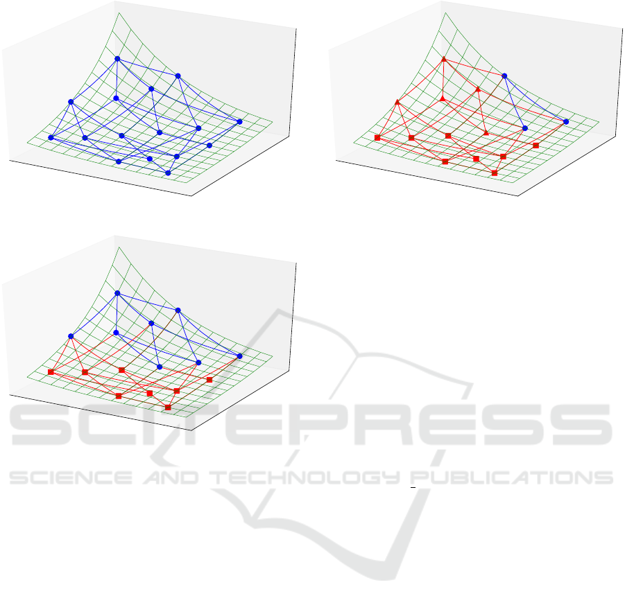
The constraint actually restricts the search space
of unsupervised feature value selection. As a result,
it leads us to one or more non-trivial local solutions,
as Fig. 3 illustrates. In the example, we assume F
b
=
{v
1
,v
2
,v
3
,v
4
} and consider the Hasse diagram of F
b
.
The Hasse diagram of F
b
is a directed graph (V
H
,E
H
)
such that V
H
is the power set of F
b
, and (S,T ) ∈ V
H
×
V
H
is in E
H
, if, and only if, S ⊃ T and |S| − |T | = 1
hold. Fig. 3 (a) depicts the Hasse diagram, and the
height of a plot of S ⊆ F
b
represents the magnitude of
H(S). On the other hand in Fig. 3 (b), the sets S ⊆ F
with supp
D
(S) 6= D are displayed in red, and we see
that there are more than one minimal selections S in
the sense that supp
D
(S) = D holds but supp
D
(T ) $ D
holds for arbitrary T $ S. One of these minimal S
is the answer to the UFVS problem. Finding exact
solutions to a UFVS problem, however, requires too
much time both in theory and in practice. We need an
approximation algorithm that works in practice.
ICAART 2020 - 12th International Conference on Agents and Artificial Intelligence
206
{v
1
, v
2
, v
3
, v
4
}
{v
2
, v
3
, v
4
}
{v
1
, v
3
, v
4
}
{v
1
, v
2
, v
4
}
{v
1
, v
2
, v
3
}
{v
3
, v
4
}
{v
2
, v
4
}
{v
2
, v
3
}
{v
1
, v
4
}
{v
1
, v
3
}
{v
1
, v
2
}
{v
4
}
{v
3
}
{v
2
}
{v
1
}
∅
(a) The Hasse diagram of {v
1
,v
2
,v
3
,v
4
}
{v
1
, v
2
, v
3
, v
4
}
{v
2
, v
3
, v
4
}
{v
1
, v
3
, v
4
}
{v
1
, v
2
, v
4
}
{v
1
, v
2
, v
3
}
{v
3
, v
4
}
{v
2
, v
4
}
{v
2
, v
3
}
{v
1
, v
4
}
{v
1
, v
3
}
{v
1
, v
2
}
{v
4
}
{v
3
}
{v
2
}
{v
1
}
∅
(b) Restriction by complete coverage
Figure 3: Search space of UFVS.
4 A NEW FAST ALGORITHM
FOR UNSUPERVISED
FEATURE VALUE SELECTION
The approximation algorithm that we propose here is
based on a gradient descent search. The following
two points are the key components of our algorithm.
1. The approximation
e
H(S) =
∑
v∈S
H(v) substitutes
for H(s);
2. A threshold parameter t is used to cut off feature
values with H(v) ≤ t before search.
The first component improves time efficiency so
that our algorithm only has to evaluate H(v) v ∈ S to
search the steepest downward edge from a selection
S ⊆ F
b
to an update. For example, in Fig. 3 (b), our
algorithm can determine whether to move from F to
F \{v
1
} by verifying only H(v
1
) > H(v
2
) > H(v
3
) >
H(v
4
), where the scores of H(v
i
) are computed once
at the beginning.
The introduction of the threshold t, on the other
{v
1
, v
2
, v
3
, v
4
}
{v
2
, v
3
, v
4
}
{v
1
, v
3
, v
4
}
{v
1
, v
2
, v
4
}
{v
1
, v
2
, v
3
}
{v
3
, v
4
}
{v
2
, v
4
}
{v
2
, v
3
}
{v
1
, v
4
}
{v
1
, v
3
}
{v
1
, v
2
}
{v
4
}
{v
3
}
{v
2
}
{v
1
}
∅
Figure 4: Restriction by a threshold.
hand, prevents the search from being captured by the
same local minimum. When we place subsets S of
the same size in increasing order of
e
H(S) from left
to right in a Hasse diagram, gradient descent always
leads us to the leftmost minimal selection. In fact,
S = {v
2
,v
3
,v
4
} is the solution of UFVS in Fig. 3 (b).
To make a move among local solutions, we introduce
the threshold parameter t, and our algorithm cuts off
the feature values v with H(v) ≤ t before starting the
search. For example, in Fig. 4, with a threshold t such
that H(v
3
) > t ≥ H(v
4
), additionally, the vertices dis-
played as red triangles are eliminated, and the solution
will be changed to {v
1
,v
3
}.
We can also frame our algorithm in the following
way. Since H(v) is an increasing function of Pr(v = 1)
if Pr(v = 1) <
1
2
, feature values v with too small H(v)
describe only a tiny portion of instances and will not
be useful to describe the dataset. For example, if v
identifies a particular instance, H(v) is the minimum.
Such feature values are eliminated by the initial cut-
off based on the threshold. On the other hand, feature
values with too great Pr(v = 1) are common among
instances and may not be useful for discriminating be-
tween instances. The gradient descent method elim-
inates feature values in the search space in decreas-
ing order of H(v), and therefore, feature values with
greater H(v) are more likely to be eliminated.
Algorithm 1 describes our algorithm. Due to the
monotonicity property of supp
D
(S) ⊆ supp
D
(T ) for
S ⊂ T , we can take advantage of a binary search to
find the next feature value to leave in S. As a result,
the algorithm is significantly fast as shown in Sec-
tion 5.1.
The time complexity of Algorithm 1 can be es-
timated as follows: the complexity of computing
H(v
i
) and the coverage of F
b
[i,|F
b
|] for all i is
O(|F
b
|·|D|); By updating the coverage of S∩F
b
[1,l]
whenever we update l, supp
D
(S \ F
b
[l + 1, j]) = D
can be investigated in O(|D|)-time, and the average
A Fast Algorithm for Unsupervised Feature Value Selection
207
complexity to execute the while loop is estimated by
O((log
2
|F
b
|)
2
· |D|).
Algorithm 1 : Unsupervised Feature Value Selection (our
algorithm).
Require: An unlabeled dataset D described by F ; a
threshold parameter t ≥ 0.
Ensure: A minimal feature value set S ⊆ F
b
.
1: Let S = F
b
\ {v
@ f
∈ F
b
| H(v
@ f
) ≤ t}.
2: Number the feature values of S so that S =
{v
1
,...,v
|S|
} and H(v
i
) ≥ H(v
j
) for i < j.
3: Let l = 0 and S = S.
4: while l < |S| do
5: Let k = max{ j | supp
D
(S\S[l +1, j]) = D, j =
l, . ..,|S|} by binary search.
6: Let S = S \ S[l + 1,k] and l = k + 1.
7: end while
8: return S.
5 EVALUATION OF
PERFORMANCE
We ran experiments to evaluate the performance of
our algorithm UFVS. In the experiments, we used the
11 datasets depicted in Fig. 1, selected from chal-
lenges of major conferences to make the evaluation
fair. The evaluation is conducted from both efficiency
and selection accuracy points of view.
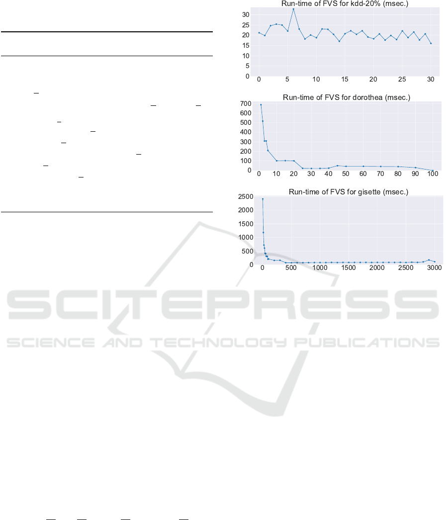
5.1 Runtime Performance
Fig. 5 describes the runtime of Algorithm 1 in mil-
liseconds for three typical datasets: KDD-20% with
significantly many instances, DOROTHEA with signif-
icantly many features, and GISETTE with both many
instances and many features (Fig. 1). The scores in-
clude only the time for search. For all 11 datasets we
investigated, the runtime is no greater than 100 mil-
liseconds, except for very small thresholds. We see
that our algorithm is extremely fast. Although the x
axis of Fig. 1 and the charts that follow it represents
the threshold t, the displayed values are the number n
with t = −
n
|D|
log
2
n
|D|
−
1 −
n
|D|
log
2
1 −
n
|D|
and
n ≤ |D|/2; for a feature value v, H(v) ≤ t, if, and only
if, the number of the instances that have v is no greater
than n.
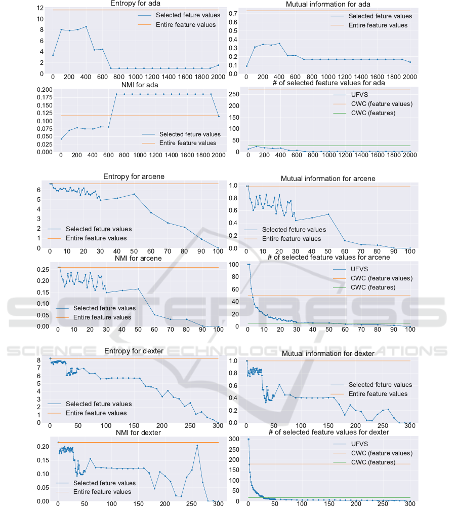
5.2 Selection Performance
Several affinities appear in the results of nine of
these eleven datasets (Fig. 6 to 10). We describe
(A) KDD-20%
(B) DOROTHEA
(C) GISETTE
Figure 5: Change in runtime measurements according to
changes in threshold t.
the affinities taking GISETTE as an example (Fig. 6).
For GISETTE, we changed the threshold t from 0 to
3,000 since GISETTE consists of 60,000 instances, the
threshold of 3,000 is as small as 5%. Fig. 8 to 10 show
the results for the other datasets.
1. The selection by our algorithm was performed
without using the label information of the dataset
at all. Even so, it found feature value sets that
can explain the labels well. In fact, I(S;C) re-
mains close to I(F ;C), until t exceeds a certain
limit (Fig 6 (b)). This property is significant ev-
idence that our algorithm has an excellent ability
to select appropriate feature values, because the
label information initially given to the datasets is
a perfect summary of the dataset.
2. Fig 6 (b) also shows that our algorithm can give
different views of the dataset by changing t. In
fact, when t exceeds the said limit, I(S;C) rapidly
decreases, and therefore, the feature values se-
lected yield different clustering results than the
initial clusters determined by the labels.
3. As t increases, I(S;C) and H(S) synchronously
decrease (Fig. 6 (a) and (b)). This can be un-
derstood, if we assume that the dataset only in-
cludes feature values relevant to the labels, and
ICAART 2020 - 12th International Conference on Agents and Artificial Intelligence
208
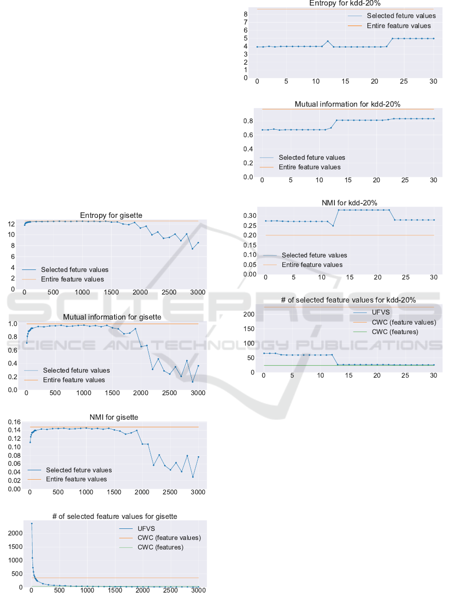
therefore, our algorithm starts to eliminate non-
redundant and relevant feature values after it has
eliminated all the redundant feature values.
4. H(S) remains very close to its upper bound H(F )
(the orange line in Fig. 6 (a)), until t reaches the
said limit. By contrast, the number of feature val-
ues selected decreases significantly rapidly as t
increases (Fig. 6 (d)). Hence, an overwhelming
majority of feature values v with small H(v) are
redundant, and eliminating them does not reduce
the information that the dataset carries.
5. Fig. 6 (d) also shows that the feature values se-
lected for t ≥ 1, 000 are fewer than the 35 features
selected by CWC (Shin et al., 2011; Shin et al.,
2015) (the green line) and significantly fewer than
the 350 feature values of these features (the or-
ange line).
(a) H(S)
(b) I(S;C)
(c) NMI(S;C)
(d) |S|
Figure 6: GISETTE.
(a) H(S)]
(b) I(S;C)
(c) NMI(S;C)]
(d) |S|
Figure 7: KDD-20%.
Also, the evaluation result of KDD-20% inter-
ests us. The dataset was created for study of intru-
sion detection. Hence, the features describe values
specified in packet headers, and the instances (pack-
ets) are annotated relating to whether they are normal
or anomalous. As opposed to the other datasets, the
score of H(S) moves around half of H(F ) (Fig. 7 (a)),
while I(S;C) remains close to I(F ;C) (Fig. 7 (b)).
In fact, KDD-20% and ADA are the only datasets
that could exhibit higher NMI(S;C) than NMI(F ;C)
(Fig. 7 (c)). With high I(S;C) and low H(S), the fea-
ture values selected could have good classification ca-
pability when used with a classifier. Also, it is sur-
prising that the number of feature values selected is
smaller than 30, when they show the highest score of
NMI(S;C). The figure is significantly lower than the
225 feature values that CWC selects for this dataset
(Fig. 7 (d)), and hence, could provide a much more
A Fast Algorithm for Unsupervised Feature Value Selection
209
ADA
ARCENE
DEXTER
Figure 8: Experimental results for ADA, ARCENE and DEXTER.
interpretable model. Although it is out of the scope
of this paper, applying our algorithm to intrusion de-
tection will be an interesting direction for future re-
search.
6 CONCLUSION
This paper introduced the principle of complete cov-
erage and formally defined unsupervised feature value
selection as an optimization problem: finding a min-
imal set of feature values that minimizes entropy un-
ICAART 2020 - 12th International Conference on Agents and Artificial Intelligence
210
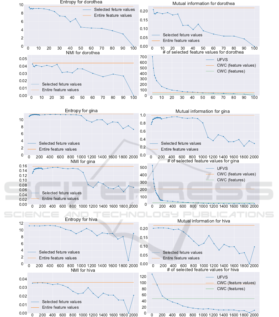
DOROTHEA
GINA
HIVA
Figure 9: Experimental results for DOROTHEA, GINA and HIVA.
der the constraint. Without the constraint, the prob-
lem has a trivial meaningless solution, and hence, the
constraint is essential to the definition of unsupervised
feature value selection. Since the problem cannot be
efficiently solved in theory and in practice, we have
proposed a fast approximation algorithm, The algo-
rithm’s efficiency makes testing a number of differ-
ent values for the threshold parameter practical, which
avoids the need for a theoretically rigorous approach.
Because no theoretically right solution for unsuper-
vised feature value selection exists, the problem is in-
tractable for unsupervised learning; by testing differ-
A Fast Algorithm for Unsupervised Feature Value Selection
211
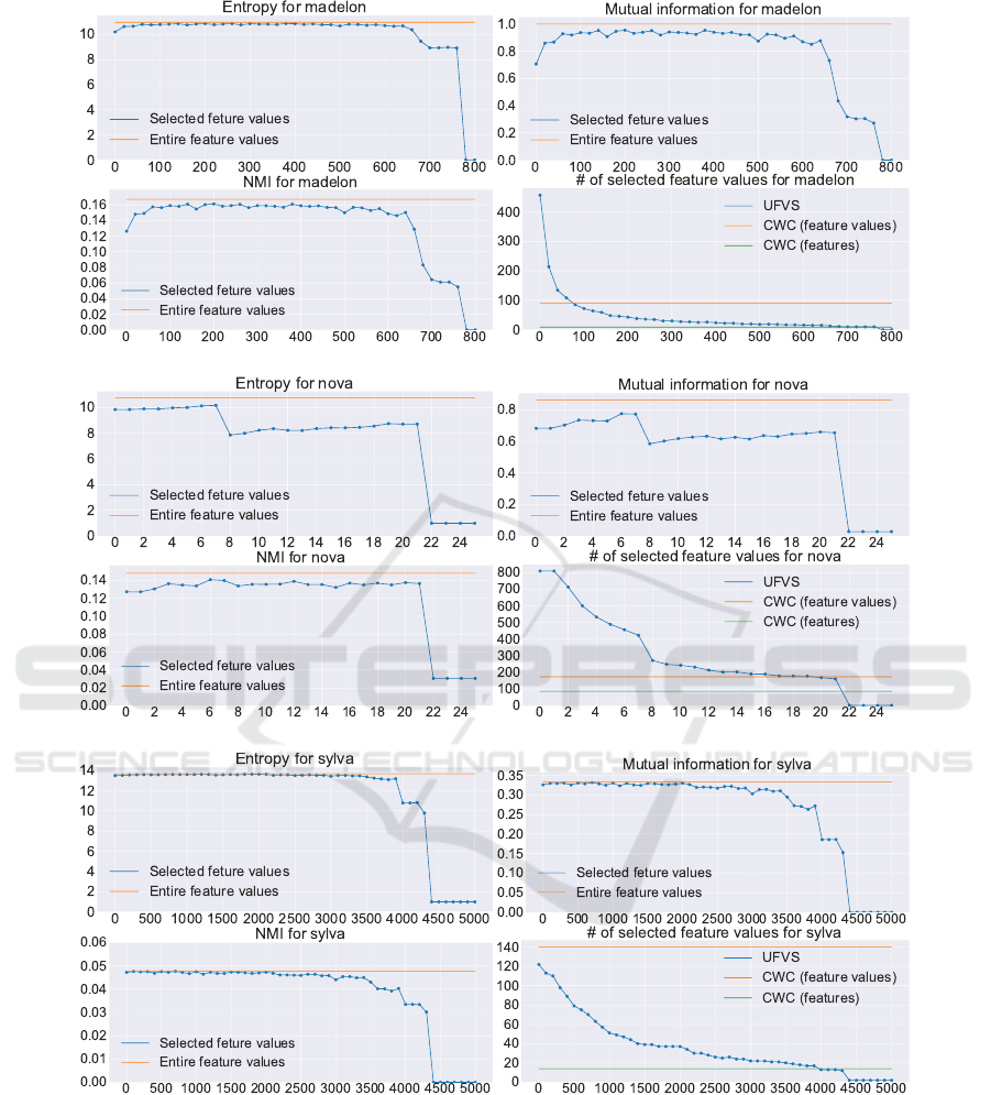
MADELON
NOVA
SYLVA
Figure 10: Experimental results for MADELON, NOVA and SYLVA.
ent threshold values, a human user is able to discover
appropriate solutions by trying a varity of different
values.
ACKNOWLEDGEMENTS
This work was partially supported by the Grant-in-
Aid for Scientific Research (JSPS KAKENHI Grant
Numbers 16K12491 and 17H00762) from the Japan
Society for the Promotion of Science.
ICAART 2020 - 12th International Conference on Agents and Artificial Intelligence
212

REFERENCES
Almuallim, H. and Dietterich, T. G. (1994). Learning
boolean concepts in the presence of many irrelevant
features. Artificial Intelligence, 69(1 - 2).
Battiti, R. (1994). Using mutual information for select-
ing features in supervised neural net learning. IEEE
Transactions on Neural Networks, 5(4):537–550.
Cai, D., Zhang, C., and He, X. (2010). In PIroceedings of
the 16th ACM SIGKDD International Conference on
Knowledge Discovery and Data Mining (KDD 2010),
pages 333–342.
Hall, M. A. (2000). Correlation-based feature selection for
discrete and numeric class machine learning. In ICML
2000.
He, X., Cai, D., and Niyogi, P. (2005). Laplacian score for
feature selection. In Advances in Neural Information
Processing Systems (NIPS 2005), pages 507–514.
LI, Z., Liu, J., Yang, Y., Zhou, X., and Liu, H. (2014).
Clustering-guided sparse structural learning for un-
supervised feature selection. IEEE Transactions on
Knowledge Data Engineering, 26(9):2138–2150.
Liu, H., Shao, M., and Fu, Y. (2016). Consensus guided
unsupervised feature selection. In Proceedings of the
28th AAAI Conference on Artificial Intelligence (AAAI
2016), pages 1874–1880.
Peng, H., Long, F., and Ding, C. (2005). Fea-
ture selection based on mutual information: Cri-
teria of max-dependency, max-relevance and min-
redundancy. IEEE Transaction on Pattern Analysis
and Machine Intelligence, 27(8).
Qian, M. and Zhai, C. (2013). Robust unsupervised feature
selection. In Proceedings of 23rd International Joint
Conference on Artificial Intelligence (IJCAI 2013),
pages 1621–1627.
Shin, K., Fernandes, D., and Miyazaki, S. (2011). Consis-
tency measures for feature selection: A formal defi-
nition, relative sensitivity comparison, and a fast al-
gorithm. In 22nd International Joint Conference on
Artificial Intelligence, pages 1491–1497.
Shin, K., Kuboyama, T., Hashimoto, T., and Shepard, D.
(2015). Super-cwc and super-lcc: Super fast feature
selection algorithms. In Big Data 2015, pages 61–67.
Shin, K., Kuboyama, T., Hashimoto, T., and Shepard, D.
(2017). sCWC/sLCC: Highly scalable feature selec-
tion algorithms. Information, 8(4).
Shin, K. and Xu, X. (2009). Consistency-based fea-
ture selection. In 13th International Conferece on
Knowledge-Based and Intelligent Information & En-
gineering System.
Wei, X., Cao, B., and Yu, P. S. (2016). Unsupervised feature
selection on networks: A generative view. In Proceed-
ings of the 28th AAAI Conference on Artificial Intelli-
gence (AAAI 2016), pages 2215–2221.
Wei, X., Cao, B., and Yu, P. S. (2017). Multi-view un-
supervised feature selection by cross-diffused matrix
alignment. In Proceedings of 2017 International Joint
Conference on Neural Networks (IJCNN 2017), pages
494–501.
Zhao, Z. and Liu, H. (2007a). Searching for interacting
features. In Proceedings of International Joint Con-
ference on Artificial Intelligence (IJCAI 2007), pages
1156 – 1161.
Zhao, Z. and Liu, H. (2007b). Spectral feature selection
for supervised and unsupervised learning. In Proceed-
ings of the 24th International Conference on Machine
Learning (ICML 2007), pages 1151–1157.
A Fast Algorithm for Unsupervised Feature Value Selection
213
