
An Economic Production Quantity Model with Imperfect Quality
Raw Material and Backorders
Noura Yassine
1
, Christine Markarian
2
and Raed El-Khalil
3
1
Department of Mathematics and Computer Science, Beirut Arab University, Beirut, Lebanon
2
Faculty of Mathematical Sciences, Haigazian University, Beirut, Lebanon
3
Information Technology and Operations Management Department, Lebanese American University, Beirut, Lebanon
Keywords: Inventory, Economic Production Model, Imperfect Quality Raw Material, Shortages, Backorder, Maximum
of Independent Random Variables.
Abstract: In this paper the classical EPQ model is extended to account for the cost and quality of the raw material used
in the production process and to incorporate the effects of shortages into the model. A production process that
uses n different types of raw material is considered. The various types of raw material acquired in batches
from the suppliers are assumed to contain a percentage of imperfect quality items of raw material. The
proportion of imperfect quality raw material found in a batch is a random variable having a known probability
distribution. A mathematical model describing the inventory/production situation is formulated and used to
derive a system of equations whose solution is the optimal production and shortage quantities that minimizes
the total cost. It is shown that the total cost function depends on the determination of the maximum of a set of
n independent random variables obtained from the proportions of imperfect quality raw material. A process
for obtaining the probability function of the maximum along with its expected value is described. Expressions
for the probability density function and the expected value of the maximum are developed for the case when
the random variables are uniformly distributed. A numerical example illustrating the determination of the
optimal policy is presented.
1 INTRODUCTION
The classical economic production quantity (EPQ)
model describes a situation where an item is produced
to meet the demand. Let denote the production rate,
the demand rate, C
0
the production setup cost, C the
unit production cost, and h the holding cost per unit
per unit time. The total inventory cost per unit time
function is given by
(
)
=+
/+ℎ1−
/2,
(1)
where Y is the quantity ordered for production at the
beginning of each production cycle. The optimal
production quantity, or the economic production
quantity, that minimizes the TCU function is
∗
=
.
(2)
Note that the classical model does not take into
account the cost or quality of the raw materials used
in the production process and considers only the cost
of the finished product. Also, the classical model
assumes that shortages are not allowed.
The classical EPQ model is based on several
assumptions that simplify the model. Numerous
research studies have extended the classical EPQ
model by relaxing some of its underlying assumptions
so that the model becomes more realistic (Yassine,
2018; Khan & Jaber, 2011). Some of the factors
introduced to relax the simplifying assumptions of the
classical EPQ model include cost of raw material
(Salameh & El-Kassar, 2007), quality of items
produced (Salameh & Jaber, 2000; Khan et al., 2011),
quality of the raw material used in the production
process (Yassine, 2016; Yassine 2018), deterioration
(Bandaly & Hassan, 2019), supply chain
considerations (Khan et al., 2011; Khan & Jaber,
2011; Bandaly et al. 2014; Bandaly et al. 2016), and
green and sustainable practices (Yassine, 2018).
202
Yassine, N., Markarian, C. and El-Khalil, R.
An Economic Production Quantity Model with Imperfect Quality Raw Material and Backorders.
DOI: 10.5220/0008980302020211
In Proceedings of the 9th International Conference on Operations Research and Enterprise Systems (ICORES 2020), pages 202-211
ISBN: 978-989-758-396-4; ISSN: 2184-4372
Copyright
c
2022 by SCITEPRESS – Science and Technology Publications, Lda. All rights reserved

Environmental concerns and resource limitations
coupled with pressure from internal and external
stakeholders have forced corporations to not only
consider efficient and effective operations (El-Khalil
& El-Kassar, 2016), but also to engage in responsible
and environmentally friendly activities. Driven by
ethical practices, engaging in responsible activities
has been shown to enhance performance (El-Kassar
& Singh, 2019; Singh et al., 2019, El-Khalil & El-
Kassar, 2018), improve governance (ElGammal et al.,
2018), and lead to employee and customer favorable
outcomes (El-Kassar et al. 2017). In addition to the
environmental and responsible practices, companies
in general and manufacturers in particular are
utilizing strategic resources, such as information and
communication technologies and innovation, for
enhancing their competitiveness level (Singh & El-
Kassar, 2019; Yunis et al., 2017; Yunis et al., 2018).
Recently, these factors have been incorporated into
the classical EPQ model (Lamba et al., 2019; Yassine,
2018).
Salameh and Jaber (2000) introduced a new
modeling approach to account for the quality of items
produced or aquired. This approach triggered a new
line of research (Khan et al., 2011; El-Kassar, 2009;
Yassine et al. 2018). Incorporating the costs and
quality of raw material used in the production process
has been the focus of several studies (Salameh & El-
Kassar, 2007; El-Kassar et al., 2012). Yassine (2018)
considered an EPQ model that takes into account the
quality of raw material; however, the model assumes
that shortages are not allowed. Yassine and
AlSagheer (2017) examined a production model with
shortages and raw materials but did not account for
the quality of the raw material.
The purpose of this paper is to extend the classical
EPQ model to account for the cost and quality of the
raw materials used in the production process and to
incorporate the effects of shortages into the model.
We consider the case that n different types of raw
material are used in the production process in which
each unit of the finished product requires one unit of
each type of raw material. At beginning of each
production/inventory cycle, the various types of raw
material are acquired in batches from the suppliers.
Each batch is assumed to contain a percentage of
imperfect quality items of raw material. The
proportion of imperfect quality raw material found in
a batch is a random variable having a known
probability.
The model also allows for shortages and
backorders and accounts for two types of shortage
cost, a constant administrative cost and a linear time
dependent cost.
A mathematical model describing the problem at
hand is formulated and used to derive a system of
equations whose solution is the optimal policy. It is
shown that the formulation of the mathematical
model depends on the determination of the maximum
of a set of n independent random variables obtained
from the proportions of imperfect quality raw
material. Thus, a process for obtaining the probability
function of the maximum along with its expected
value is described. Moreover, expressions for the
probability density function and the expected value of
the maximum are developed for the case when the
random variables are uniformly distributed. The
results are then applied to the EPQ model considered
in this paper. A numerical example illustrating the
determination of the optimal policy is presented.
The rest of this paper is organized in the following
manner. In section 2, the mathematical model is
formulated. The determination of the distribution and
the expectation of the maximum of a set of
independent random variables is discussed in section
3. In section 4, a case is presented to illustate the
calculation of optimal solution. The paper concludes
in section 5.
2 MATHEMATICAL MODEL
In this section, the mathematical model describing the
problem at hand is formulated and used to derive a
system of equations whose solution is the optimal
policy.
2.1 Notation
The following notation is used throughout the rest of
this paper:
Y Order size of finished product
S Size of planned shortage
M Maximum inventory level
U
j
Order size of raw material of type j
Α Production rate
β Demand rate
C
0
Production set up cost
C
p
Unit production cost
C
j
Ordering cost of raw material of type j
C
rj
Unit purchasing cost of raw material of
type j
C
dj
Screening cost per unit of raw material of
type j
An Economic Production Quantity Model with Imperfect Quality Raw Material and Backorders
203

C
b
Administrative cost per unit short of the
finished product
C
s
Cost per unit short of the finished product
per unit time
h
rj
Holding cost per unit of raw material of
type j per unit time
h
P
Holding cost per unit of finished product
per unit time
γ
j
Screening rate of raw material of type j
j
Percentage of imperfect quality of raw
material of type j
g
j
(
j
) Probability density function of
j
µ
j
Expected value of
j
S
rj
Salvage value per unit of imperfect quality
raw material of type j
Tp Length of the production period
T Length of the inventory cycle
T
1
Time to fulfil the backorder of size S
T
2
Time to build the maximum inventory
level
T
3
Time to deplete the maximum inventory
T
4
Time to build a backorder of size S
2.2 Problem Formulation
Let Y be the order size of the finished product, an
unknown to be determined by minimizing the total
cost per unit time function. At the start of each
production cycle, the various types of raw material
acquired from the suppliers are processed into a
finished product at a production rate . The batch of
raw material of type j acquired from supplier j is
screened for imperfect quality items at a rate
j
. The
screening period is U
j
/
j
, where U
j
is the order size of
raw material of type j. Suppose that is
U
j
= Y/(1
µ
j
),
(3)
where µ
j
is the expected value of
j
, the proportion of
imperfect quality raw material of type j. From Eq. (3),
the amount of perfect quality raw material of type j is
(1
j
)U
j
= (1
j
)Y/(1 µ
j
),
(4)
so that its expected value is
E[(1
j
)U
j
] = E[1
j
]Y/(1 µ
j
) = Y.
(5)
On the other hand, the amount of imperfect quality
raw material of type j is
j
U
j
=
j
Y/(1 µ
j
),
(6)
and its expected value is
E[
j
U
j
] = E[
j
Y/(1
µ
j
)] = µ
j
Y/(1 µ
j
).
(7
)
Since each unit of the finished product requires
exactly one unit of perfect quality raw material of
type j, U
j
must be larger than the order size of the
finished product Y. Note that the imperfect quality of
raw material of type j is accounted for as follows:
=
=
=+
.
(8
)
The additional amount ordered is exactly the expected
amount of imperfect quality of raw material of type j.
However, the actual amount of perfect quality raw
material may differ. Let Z
j
denote this difference.
From Eqs. (6) and (7),
=
−
=
.
(9
)
This difference determines the number of finished
items produced using the perfect quality raw material
received during the current production cycle. Let W
c
denote this number. Then,
W
c
= Y
Max{Z
j
: 1 ≤ j ≤ n}
= Y
YMax{(
j
µ
j
)/(1 µ
j
)
: 1 ≤ j ≤ n}.
(10
)
Hence, the determination of the optimal production
quantity depends on calculating the maximum of the
n independent continuous random variables
=
.
(11
)
Note that each of these variables has a mean of 0.
Define the expected value of the maximum of
X
1
, X
2
, …, X
n
to be
µ = E[Max{X
j
: 1 ≤ j ≤ n}]. (12
)
The value of µ depends on the distribution of the
variables X
j
, 1 ≤ j ≤ n. In section 3, we consider the
case where the random variables
1
,
2
, …,
n
are
uniformly distributed.
From Eq. (10), the expected number of finished
items produced using the perfect quality raw
materials received during the current cycle is
E[W
c
] = Y(1
µ).
(13
)
ICORES 2020 - 9th International Conference on Operations Research and Enterprise Systems
204

Note that, from Eqs. (4) and (10), the number of
unused good quality items of raw material of type j
received during the current cycle is
=
(1−
)
1−
−
.
(14)
Using Eqs. (5) and (13), the expected number of
unused good quality items of type j raw material is
=
−
(
1−
)
=.
(15)
The on-hand good quality raw materials are processed
at a rate until the end of the production period. The
length of the production period is
=/,
(16)
where W is the total number of items produced during
the current production cycle using both the perfect
quality raw materials received at the beginning of the
inventory cycle as well as the excess perfect quality
raw materials kept in stock from previous cycles. Let
W
p
be the number of finished items produced using
the excess perfect quality raw materials kept in stock
from previous cycles. Hence, W = W
c
+W
p
.
Since each excess amount has the same expected
value of E[e
j
] = µY, the expected number of finished
product produced using the excess amount is also µY.
Hence, the expected total number of finished product
produced during a production cycle is exactly the
order quantity Y. That is,
E[W] = E[W
c
+W
p
] = Y(1µ)+µY = Y.
(17)
From Eqs. (16) and (17), the expected length of
the production cycle is
E[T
p
] = E[W/
]=Y/.
(18)
During the production period, items of the
finished product are produced at a rate and used at
a rate to meet the demand. At the start of the
production period and until time T
1
, the excess
amount of the finished product is used to fulfil the
backorders at a rate of . Hence,
T
1
= S/(
).
(19)
After such time and until the end of the production
period, the excess amount of the finished product is
used to accumulate finished product inventory at a
rate of . This occurs during a time period of T
2
,
where T
p
= T
1
+T
2
. Hence,
T
2
=T
P
T
1
=
W
/
S
/(
)
.
(20
)
At the end of this period, a maximum inventory level
M is reached. Then,
=
(
−
)
=
(
1−/
)
−.
(21
)
This maximum level will be used to meet the demand
at a rate until time T
3
, when the inventory level of
the finished product reaches zero. Hence,
=
=
(
/
)
=
1−
−
.
(22
)
Throughout the remainder of the inventory cycle,
a planned shortage of size S is accumulated at a rate
during a time period of T
4
, where
=/.
(23
)
The finished product inventory level is shown in Fig.
1. Note that the length of the inventory cycle is T = T
1
+ T
2
+ T
3
+ T
4
. Eqs. (19), (20), (22) and (23) give that
=/.
(24
)
From Eqs. (13) and (24), the expected inventory
length is
[
]
=/.
(25
)
2.3 The Cost Function
The optimal production quantity Y
*
and the optimal
shortage quantity S
*
are determined by minimizing
the total cost per unit time function given by
(
,
)
=
(
,
)
,
(26
)
where TC(Y, S) is the total cost per inventory cycle
function. The TC(Y, S) function comprises of the
following cost components:
Ordering, purchasing, screening and holding
costs of raw material.
Setup cost of production.
Production and holding costs of finished product.
Shortage and backorder costs.
An Economic Production Quantity Model with Imperfect Quality Raw Material and Backorders
205
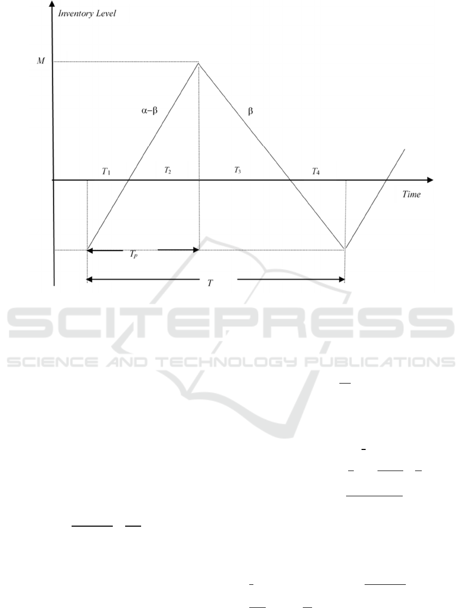
Figure 1: Finished Product Inventory level.
The ordering cost of raw materials of type j is C
j
and the purchasing cost is C
rj
U
j
. The purchasing cost
of raw material is reduced by an amount S
rj
j
U
j
,
which is the salvage value resulting from discarding
the imperfect quality items at a discount price. Fig. 2
depicts the inventory level of raw material. Note that
the drop in inventory level represents the selling of
the
j
U
j
imperfect quality items of raw material.
The raw materials holding cost is the holding cost
per unit of raw material per unit time, namely h
rj
,
multiplied by the average on hand inventory of raw
material times the cycle length. That is, h
rj
multiplied
by the area under the curve in Fig. 2. Hence, the total
holding cost of raw material per inventory cycle is
RawMaterialHoldingCost=
∑
ℎ
+
+
.
(27)
The cost of producing the W units of the finished
product is the sum of the setup C
0
and the variable
production cost given by C
p
W. The holding cost per
unit of the finished product per unit time is h
p
. Thus,
the finished product holding cost is the average
inventory of on hand finished product times the
inventory cycle length times the holding cost per unit
per unit time, which is h
p
times the area in Fig. 1 under
the curve and above the x-axis. Using Eqs. (20) to
(22),
FinishedProductholdingCost
=
ℎ
2
..
(
+
)
.
(28)
From Fig. 1 and using Eqs. (19) to (23), the shortage
cost is
ShortageCost=
+
(
+
)
.
(29
)
=
+
1
2
−
+
=
+
2(1−/)
.
Hence, the total inventory cost per cycle is
(
,
)
=
+
∑
+
∑
+
−
+
+
+
(
+
)
+
∑
ℎ
+
+
+
..
(
+
)
.
(30
)
ICORES 2020 - 9th International Conference on Operations Research and Enterprise Systems
206
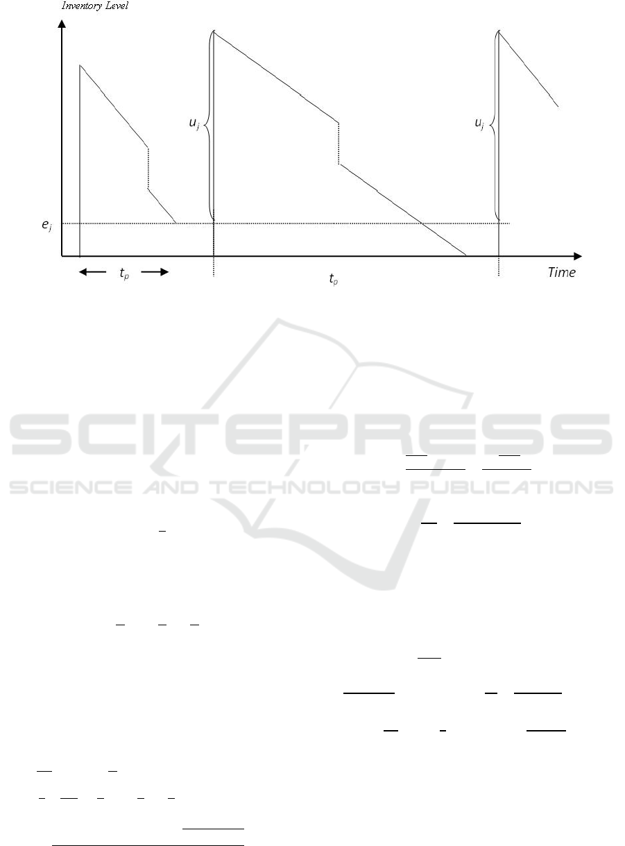
Figure 2: Inventory level of raw material of type j component.
The next step is to determine the expected total cost
per inventory cycle. For this purpose, we note that in
a typical inventory cycle, depicted in Fig. 1, the
expected time required to build up the maximum
inventory of finished items obtained using Eqs. (17)
and (20) is
E
[
T
2
]
=
Y
/
S
/(
)
.
(31)
Similarly, Eqs. (17) and (21) give the expected
maximum inventory of finished items as
[
]
=1−
−.
(32)
Also, the expected time to deplete the maximum
inventory is obtained from Eqs. (17) and (22) as
[
]=
1−
−
.
(33)
The area under the curve in Fig. 1 representing the
on-hand inventory of the finished product is used to
calculate the expected holding cost of the finished
product. From Eqs. (28) and (31) to (33), we have
ExpectedFinishedProductHoldingCost
(34
)
=
ℎ
2
.1−
−
.
+
1−
−
=ℎ
(1−/)
−2+
(1−/)
2
.
Similarly, during a typical cycle, the expected
area under the curve representing the on-hand
inventory of the raw material of type j can used to
calculate the expected total holding cost of the raw
material. From Eqs. (15), (18) and (27), we have
ExpectedRawMaterialHoldingCost=
∑
ℎ
+
+
(35
)
=ℎ
2
+
1−
+
The expected total inventory cost per cycle ETC(Y,S)
= E[TC(Y, S)] obtained by taking the expected value
of the various costs in Eq. (30) is
(
,
)
=
+
∑
+
∑
+
−
+
+
+
(/)
+
∑
ℎ
+
+
+
1−
−2+
(/)
.
(36
)
The expected total inventory cost per unit time,
ETCU(Y,S) = E[TCU(Y, S)] = E[TC(Y, S)/T], is
approximated using the Renewal Reward Theorem as
ETCU(Y,S) = E[TC(Y, S)]/ E[T]. Dividing Eq. (36) by
the expected cycle length T given by Eq. (25). Hence,
An Economic Production Quantity Model with Imperfect Quality Raw Material and Backorders
207

(
,
)
=
+
∑
+
+
(/)
+
∑
+
−
+
+
∑
ℎ
+
++
1−
−2+
(/)
.
(37)
Note that the expected total cost per unit function
depends on the determination of the expected value µ
of the maximum of the random variables in X
1
, X
2
, …,
X
n
. In section 3, the calculation of µ is described in
the case where the random variables are uniformly
distribution.
2.4 The Optimal Solution
To obtain the optimal production quantity Y
*
and the
optimal shortage size S
*
, we find the first partial
derivatives of ETCU(Y, S) and set these derivatives
equal to zero. Differentiating ETCU(Y, S) with
respect to S, we get
(
,
)
=
+
(1−/)
(38)
+ℎ
−1+
(1−/)
Y
.
Setting the derivative in Eq. (38) equal to zero and
rearranging, we get
ℎ
−
(
)
(/)
−
= 0.
(39)
Now we differentiate ETCU(Y, S) with respect to Y,
we get
(
,
)
=−
+
∑
+
+
+
∑
ℎ
+
+
1−
−
.
(40)
Setting the derivative in Eq. (40) to zero and
rearranging, we have
−2
+
∑
+
+
ℎ
1−
+2
∑
ℎ
+
−
=0.
(41)
The solution of the system of equations (39) and
(41) provide the optimal production quantity Y
*
and
optimal shortage quantity S
*
. Note that the second
partial derivatives obtained from (38) and (40) may
be used to either demonstrate the uniqueness of the
optimal solution or provide conditions that guarantee
it. In the following section, we describe how the
expected value of the maximum of a set of
independent random variables can be calculated.
3 MAXIMUM OF A SET OF
RANDOM VARIABLES
Functions of random variables have many
applications in various fields, see (Yassine, 2018;
Yassine and El-Rabih, 2019). The optimal solution
derived in section 2 depends on the exepected value
of the maximum of random variables each having a
mean equal to 0. Hence, a process for obtaining the
probability function of the maximum along with its
expected value is needed. In the following, we
describe such a process based argumentes similar to
those Yassine (2018) used to determine the
probability distribution and expected value of the
minimum of uniformly distributed random variables
each having a mean equal to 1.
Let X
1
, X
2
,…, X
n
be n independent continuous
random variables and let g
j
(X
j
) denote the probability
distribution of X
j
. Since X
1
, X
2
, …, X
n
are
independent, the cumulative distribution of the
random variable Max(X
1
, X
2
, …, X
n
) is
(
)
=
(
(
,
,…,
)≤
)
(42)
=
(
≤
)
(
≤
)
…
(
≤
)
=
(
)
.
(
)
…
(
)
,
where G
j
(t) is the cumulative distribution of X
j
.
In the case where each X
j
is uniformly distributed over
an interval [m
j
, m
j
] centered at zero, the probability
distribution of X
j
is
=
0
<−
1
2
−
≤
≤
0
>
,
(43)
ICORES 2020 - 9th International Conference on Operations Research and Enterprise Systems
208
and its cumulative distribution, a continuous function,
is
(
)
=
0≤−
+
2
−
≤≤
1≥
.
(44)
Since each interval [m
j
, m
j
] is centered at 0, we may
assume, without loss of generality, that these intervals
are nested so that
m
n
≤…≤m
2
≤m
1
≤ 0 ≤ m
1
≤m
2
≤…
≤ m
n
.
(45)
From Eqs. (42) and (44), the cumulative distribution
of the maximum is
(
)
=
0
∏
≤−
−
≤≤
∏
≤≤
1≥
.
(46)
The expected value µ of Max(X
1
, X
2
,…, X
n
) is
calculated using
μ= ℎ
(
)
,
(47)
where h(t) is the derivative of H(t).
In case when n = 2, the cumulative distribution in
Eq. (46) reduces to
(
)
=
0≤−
(
)(
)
−
≤≤
≤≤
1≥
,
(48)
and the probability density function h(t) of Max(X
1
,
X
2
,…, X
n
) is
ℎ
(
)
=
0<−
−
≤<
≤≤
0>
.
(49)
Hence,
=
(
2+
+
)
4
(50)
+ /(2
)=
12
+
4
.
When each
j
is uniformly distributed over an
interval [a
j
, b
j
], the random variable X
j
is also
uniformly distributed over an interval centred at 0,
say [m
j
, m
j
], where
=
=
(
)/
(
)/
=
.
(51
)
4 NUMERICAL EXAMPLE
Consider a production process where the demand rate
for an item is 100 units per day and the production
rate is 400 units per day. Assume that the percentage
of imperfect raw material of type 1 used in production
is uniformly distributed over [10%, 30%] so that the
mean is 20%. Similarly, the percentage of imperfect
raw material of type 2 is uniformly distributed over
[10%, 40%] so that the mean is 25%. Screening for
imperfect quality items of the raw material of type 1
is conducted at a rate of 1200 units per day and at a
cost of $0.20 per unit, and for type 2 at a rate of 800
units per day and at a cost of $0.25 per unit. The
ordering cost for the raw material of type 1 is $2,000,
of type 2 is $3,000, and the production setup cost is
$4750. The holding cost of raw material of type 1 is
$0.2 per unit per day and $0.3 per unit per day for raw
material of type 2. The holding cost per unit of the
finished product per day is $0.92. The production cost
is $ 30 per unit. The purchasing cost of one item of
raw material of type 1 is $10 and $20 for type 2.
Planned shortages are permitted. The cost of having
one finished short is $2.6 per day and the
administrative cost of a unit short is $10. The
production cost per unit is $30. The Salvage value per
unit of imperfect quality raw material of type 1 is $5
and $10 for type 2.
The parameters of the problem are α = 400, =
100, C
0
= 4750, C
p
= 30, C
1
= 2000, C
2
= 3000, C
r1
=
10,
C
r2
= 20,
C
d1
= 0.2,
C
d2
= 0.25,
C
b
= 10, C
s
= 2.6,
h
r1
= 0.2,
h
r2
= 0.3,
h
P
= 0.92,
γ
1
= 1200,
γ
2
= 800, S
r1
= 5,
S
r2
= 20,
1
[10%, 30%], a
1
= 0.10, b
1
= 0.30, g
1
(
1
)
= 1/(0.30.1) = 5;
1
= (0.1+0.3)/2 = 0.2;
2
[10%,
40%]; a
2
= 0.10, b
2
= 0.40, g
2
(
2
) = 1/(0.40.1) =
3.33;
2
= (0.1+0.4)/2 = 0.25.
To determine the optimal production policy, first
we need to determine the random variables X
1
, X
2
, and
Max(X
1
, X
2
). Also, the expected value µ = E(Max(X
1
,
X
2
)) needs to be calculated. From Eq. (51), the value
An Economic Production Quantity Model with Imperfect Quality Raw Material and Backorders
209

of m
1
is obtained as m
1
= (0.30.1)/(20.10.3) =
0.125. Hence, X
1
is uniformly distributed over
[0.125, 0.125]. Similarly, m
2
=
(0.40.1)/(20.10.4) = 0.2 so that X
2
is uniformly
distributed over [0.2, 0.2]. The expected value of
Max(X
1
, X
2
) can now be calculated using Eq. (50) as
µ =
.
(.)
+
.
= 0.05651.
Solving the system in Eqs. (39) and (41) results in
two solutions. The first has negative values for S and
Y, which is rejected. The second solution gives the
optimal production quantity Y
*
= 1600.09 1600
and the optimal shortage quantity S
*
= 100.59 100.
Then, ETCU(1600, 100) = 7801.03. The order
quantity of raw material of type 1 is U
1
= Y/(1
1
)
=1600/(10.8) = 2000. Similarly, U
2
= Y/(1
2
)
=1600/(10.75) = 2133. The expected number of
finished items produced from the raw materials
obtained during the current production cycle is E[W
c
]
= Y(1µ) = 1510. Also, the expected number of
finished items produced from the excess perfect
quality raw material kept in stock from previous
periods is E[W
p
] = E[e
1
] = E[e
2
] = µY = 90.
The expected cycle length and production period
are E[T] = 1600/100 = 16 and E[T
p
] = 1600/400 = 4.
The maximum inventory level of the finished product
is E[M] = 1600(1100/400) 100 = 1100.
5 CONCLUSION
In this paper, an economic production model that
accounts for the cost and quality of the raw materials
was presented. Also, the effects of shortages were
incorporated into the model. A mathematical model
describing this production/inventory situation was
formulated. It was shown that the optimal production
and shortage quantities that minimize the total
inventory cost per unit time function are the solution
of a system of equations derived using the
mathematical model. The total cost function was
shown to depend on the maximum of a set of n
independent random variables obtained from the
proportion of imperfect quality raw material.
A process for obtaining the probability function of
the maximum and its expected value was developed
and described. Moreover, expressions for the
probability density function and the expected value of
the maximum when the random variables are
uniformly distributed were obtained. The results were
applied to the EPQ model considered in this paper. A
numerical example illustrating the determination of
the optimal policy was presented.
This study has some limitations. Due to the
restriction on the length of the paper, uniqueness of
the optimal solution was not demonstrated nor
sensitivity analysis was performed. Also, the model
considered the producer as the decision maker and
ignored the other supply chain members. These
limitations can be tackled in future research.
REFERENCES
Bandaly, D. C., & Hassan, H. F. (2019). Postponement
implementation in integrated production and inventory
plan under deterioration effects: a case study of a juice
producer with limited storage capacity. Production
Planning & Control, 1-17.
Bandaly, D., Satir, A., & Shanker, L. (2016). Impact of lead
time variability in supply chain risk
management. International Journal of Production
Economics, 180, 88-100.
Bandaly, D., Satir, A., & Shanker, L. (2014). Integrated
supply chain risk management via operational methods
and financial instruments. International Journal of
Production Research, 52(7), 2007-2025.
ElGammal, W., El-Kassar, A. N., & Canaan Messarra, L.
(2018). Corporate ethics, governance and social
responsibility in MENA countries. Management
Decision, 56(1), 273-291.
El-Kassar, A. N. M. (2009). Optimal order quantity for
imperfect quality items. In Allied Academies
International Conference. Academy of Management
Information and Decision Sciences. Proceedings (Vol.
13, No. 1, p. 24). Jordan Whitney Enterprises, Inc.
El-Kassar, A. N., Salameh, M., & Bitar, M. (2012) EPQ
model with imperfect quality raw material.
Mathematica Balkanica, 26, 123-132.
El-Kassar, A. N., Yunis, M., & El-Khalil, R. (2017). The
mediating effects of employee-company identification
on the relationship between ethics, corporate social
responsibility, and organizational citizenship
behavior. Journal of Promotion Management, 23(3),
419-436.
El-Kassar, A. N., & Singh, S. K. (2019). Green innovation
and organizational performance: the influence of big
data and the moderating role of management
commitment and HR practices. Technological
Forecasting and Social Change, 144, 483-498.
El-Khalil, R., & El-Kassar, A. N. (2016). Managing span of
control efficiency and effectiveness: a case
study. Benchmarking: An International Journal, 23(7),
1717-1735.
El-Khalil, R., & El-Kassar, A. N. (2018). Effects of
corporate sustainability practices on performance: the
case of the MENA region. Benchmarking: An
International Journal, 25(5), 1333-1349.
Khan, M., Jaber, M.Y., Guiffrida, A.L., and Zolfaghari, S.
(2011) A review of the extensions of a modified EOQ
model for imperfect quality items, International
Journal of Production Economics 132 (1), 1-12.
ICORES 2020 - 9th International Conference on Operations Research and Enterprise Systems
210

Khan, M., and Jaber, M.Y. (2011) Optimal inventory cycle
in a two-stage supply chain incorporating imperfect
items from suppliers, Int. J. Operational Research
10(4), 442–457.
Lamba, K., Singh, S. P., & Mishra, N. (2019). Integrated
decisions for supplier selection and lot-sizing
considering different carbon emission regulations in
Big Data environment. Computers & Industrial
Engineering, 128, 1052-1062.
Salameh, M. K., & El-Kassar, A. N. (2007, March).
Accounting for the holding cost of raw material in the
production model. In Proceeding of BIMA inaugural
conference (pp. 72-81).
Salameh, M. K., and Jaber, M. Y. (2000) Economic
production quantity model for items with imperfect
quality, International Journal of Production Economics
64, 59–64.
Singh, S. K., & El-Kassar, A. N. (2019). Role of big data
analytics in developing sustainable capabilities. Journal
of cleaner production, 213, 1264-1273.
Singh, S. K., Chen, J., Del Giudice, M., & El-Kassar, A. N.
(2019). Environmental ethics, environmental
performance, and competitive advantage: Role of
environmental training. Technological Forecasting and
Social Change, 146, 203-211.
Yassine, N. (2016) Joint Probability Distribution and the
Minimum of a Set of Normalized Random Variables,
Procedia - Social and Behavioral Sciences, 230 (12),
235–239.
Yassine, N. & AlSagheer, A. (2017). The optimal solution
of a production model with shortages and raw
materials. Int J Math Comput Methods, 2, 13-18.
Yassine, N. (2018). A sustainable economic production
model: effects of quality and emissions tax from
transportation. Annals of Operations Research, 1-22.
Yassine, N., AlSagheer, A., & Azzam, N. (2018). A
bundling strategy for items with different quality based
on functions involving the minimum of two random
variables. International Journal of Engineering
Business Management, 10, 1-9.
Yassine, N., & El-Rabih, S. (2019, May). Assembling
Components with Probabilistic Lead Times. In IOP
Conference Series: Materials Science and Engineering
(Vol. 521, No. 1, p. 012013).
Yunis, M., Tarhini, A., & Kassar, A. (2018). The role of
ICT and innovation in enhancing organizational
performance: The catalysing effect of corporate
entrepreneurship. Journal of Business Research, 88,
344-356.
Yunis, M., El-Kassar, A. N., & Tarhini, A. (2017). Impact
of ICT-based innovations on organizational
performance: The role of corporate
entrepreneurship. Journal of Enterprise Information
Management, 30(1), 122-141.
An Economic Production Quantity Model with Imperfect Quality Raw Material and Backorders
211
