On Satisﬁsﬁability Modulo Theories in

Continuous Multi-Agent Path Finding: Compilation-based and

Search-based Approaches Compared

Pavel Surynek

Faculty of Information Technology, Czech Technical University in Prague, Th

akurova 9, 160 00 Praha 6, Czech Republic

pavel.surynek@ﬁt.cvut.cz

Keywords:

Multi-Agent Path Finding (MAPF), Satisﬁability Modulo Theory (SMT), Continuous Time, Continuous

Space, Makespan Optimal Solutions, Geometric Agents.

Abstract:

Multi-agent path ﬁnding (MAPF) in continuous space and time with geometric agents, i.e. agents of various

geometric shapes moving smoothly between predeﬁned positions, is addressed in this paper. We analyze

a new solving approach based on satisﬁability modulo theories (SMT) that is designed to obtain makespan

optimal solutions. The standard MAPF is a task of navigating agents in an undirected graph from given

starting vertices to given goal vertices so that agents do not collide with each other in vertices or edges of

the graph. In the continuous version (MAPF

), agents move in a metric space along predeﬁned trajectories

that interconnect predeﬁned positions. Agents themselves are geometric objects of various shapes occupying

certain volume of the space - circles, polygons, etc. For simplicity, we work with circular omni-directional

agents having constant velocities in the 2D plane where positions are interconnected by straight lines. As

agents can have different shapes/sizes and are moving smoothly along lines, a movement along certain lines

done with small agents can be non-colliding while the same movement may result in a collision if performed

with larger agents. Such a distinction rooted in the geometric reasoning is not present in the standard MAPF.

The SMT-based approach for MAPF

called SMT-CBS

reformulates the well established Conﬂict-based

Search (CBS) algorithm in terms of SMT. Lazy generation of decision variables and constraints is the key

idea behing SMT-CBS. Each time a new conﬂict is discovered, the underlying encoding is extended with new

variables and constraints to eliminate the conﬂict. We compared SMT-CBS

and adaptations of CBS for the

continuous variant of MAPF experimentally.

1 INTRODUCTION AND

BACKGROUND

In multi-agent path ﬁnding (MAPF) (Kornhauser

et al., 1984; Ryan, 2008; Sharon et al., 2015; Sharon

et al., 2013a; Silver, 2005; Surynek, 2009; Wang and

Botea, 2011) the task is to navigate agents from given

starting positions to given individual goals. The prob-

lem takes place in undirected graph G = (V,E) where

agents from set A = {a

,...,a

} are placed in ver-

tices so that there is at most one agent per vertex. The

initial conﬁguration of agents in vertices of the graph

can be written as simple assignment α

: A → V and

similarly the goal conﬁguration as α

: A → V . The

task of navigating agents can be then expressed as a

task of transforming the initial conﬁguration of agents

: A → V into the goal conﬁguration α

: A → V .

In the standard MAPF, movements are instanta-

neous and are usually possible into vacant neighbors

assuming no other agent is entering the same tar-

get vertex

. We usually denote the conﬁguration of

agents at discrete time step t as α

: A → V . Non-

conﬂicting movements transform conﬁguration α

in-

stantaneously into next conﬁguration α

t+1

so we do

not consider what happens between time steps t and

t + 1.

In order to reﬂect various aspects of real-life appli-

cations variants of MAPF have been introduced such

as those considering kinematic constraints (H

onig

et al., 2017), large agents (Li et al., 2019), or dead-

lines (Ma et al., 2018) - see (Ma et al., 2017) for

more variants. Particularly in this work we are deal-

ing with an extension of MAPF introduced only re-

cently (Andreychuk et al., 2019b; Andreychuk et al.,

Different versions of MAPF permit entering a vertex

being simultaneously vacated by another agent excluding

the trivial case when agents swap their position across an

edge.

2019a; Walker et al., 2018) that considers contin-

uous time and space and continuous movements of

agents between predeﬁned positions placed arbitrar-

ily in the metric space. The continuous version will

be denoted as MAPF

. It is natural in MAPF

assume geometric agents of various shapes that oc-

cupy certain volume in the space - circles in the 2D

space, polygons, spheres in the 3D space etc. In con-

trast to MAPF, where the collision is usually deﬁned

as the simultaneous occupation of a vertex by two

(or more) agents, collisions are deﬁned as any spa-

tial overlap of agents’ bodies in MAPF

. Agents in

MAPF

move along predeﬁned trajectories that in-

terconnects predeﬁned positions. Assuming certain

individual speed of an agent we can assign the agent a

position in the space at any moment. Different shapes

of agents’ bodies play a role. Hence for example a

movement along two distinct trajectories that is colli-

sion free when done with small agents may turn into

a collision if performed with large agents. For sim-

plicity we will assume agents moving along straight

lines but the the presented techniques are applicable

to different trajectories as well.

The motivation behind introducing MAPF

is the

need to construct more realistic paths in many appli-

cations such as controlling ﬂeets of robots or aerial

drones (Janovsky et al., 2014; C

ap et al., 2013) where

continuous reasoning is closer to the reality than the

standard MAPF.

The contribution of this paper consists in show-

ing how to apply satisﬁability modulo theory (SMT)

reasoning (Boﬁll et al., 2012; Nieuwenhuis, 2010) in

MAPF

solving. The SMT paradigm constructs deci-

sion procedures for various complex logic theories by

decomposing the decision problem into the proposi-

tional part having arbitrary Boolean structure and the

theory part that is restricted on the conjunctive frag-

ment.

1.1 Related Work and Organization

Our SMT-based approach focuses on makespan opti-

mal MAPF solving and builds on top of the Conﬂict-

based Search (CBS) algorithm (Sharon et al., 2012;

Sharon et al., 2015). Makespan optimal solutions

minimize the overall time needed to relocate all

agents into their goals.

CBS tries to solve MAPF lazily by adding con-

ﬂict elimination constraints on demand. It starts with

the empty set of constraints. The set of constraints is

iteratively reﬁned with new conﬂict elimination con-

straints after conﬂicts are found in solutions for the in-

complete set of constraints. Since conﬂict elimination

constraints are disjunctive (they forbid occurrence of

one or the other agent in a vertex at a time) the reﬁne-

ment in CBS is carried out by branching in the search

process.

CBS can be adapted for MAPF

by implement-

ing conﬂict detection in continuous time and space

while the high-level framework of the CBS algorithm

remains the same as shown in (Andreychuk et al.,

2019b; Andreychuk et al., 2019a).

In the SMT-based approach we are trying to build

an incomplete propositional model so that if a given

MAPF

has a solution of a speciﬁed makespan

then the model is solvable (but the opposite impli-

cation generally does not hold). This is similar to

the previous SAT-based (Biere et al., 2009) MAPF

solving (Surynek, 2012; Surynek et al., 2016) where

a complete propositional model has been constructed

(that is, the given MAPF has a solution of a speciﬁed

makespan if and only is the model is solvable).

The propositional model in the SMT-based ap-

proach in constructed lazily through conﬂict elimina-

tion reﬁnements as done in CBS. The lazy approach

of propositional model construction for the standard

MAPF was ﬁrst introduced in (Surynek, 2019). Here

we further generalize the SMT-based approach for

MAPF

. Similar techniques for lazy introduction of

constraints are also known in integer programming

and were succesfully applied in the standard MAPF

solving as well (Lam et al., 2019).

The incompleteness of the model is inherited from

CBS that adds constraints lazily. This is in contrast to

SAT-based methods like MDD-SAT (Surynek et al.,

2016) where all constraints are added eagerly result-

ing in a complete model. We call our new algorithm

SMT-CBS

. The major difference of SMT-CBS

from CBS is that instead of branching the search we

only add a disjunctive constraint to eliminate the con-

ﬂict in SMT-CBS

. Hence, SMT-CBS

does not

branch the search at all at the high-level. The proposi-

tional model is incrementally reﬁned at the high-level

instead.

Similarly as in the SAT-based MAPF solving we

use decision propositional variables indexed by agent

a, vertex v, and time t with the meaning that if the

variable is TRUE agent a appears in v at time t. How-

ever the major technical difﬁculty with the continuous

version of MAPF is that we do not know all necessary

decision variables in advance due to continuous time.

After a conﬂict is discovered we may need new de-

cision variables to avoid that conﬂict. For this reason

we introduce a special decision variable generation al-

gorithm that generates decision variables on demand.

The paper is organized as follows: we ﬁrst intro-

duce MAPF

formally. Then we recall a variant of

CBS for MAPF

. Details of the novel SMT-based

solving algorithm SMT-CBS

follow. Finally, an ex-

perimental evaluation of SMT-CBS

against the con-

tinuous version of CBS is shown. We also show a

brief comparison with the standard MAPF.

1.2 MAPF with Continuous Time

We follow the deﬁnition of MAPF with continu-

ous time denoted MAPF

from (Andreychuk et al.,

2019b) and (Walker et al., 2018). MAPF

several components with the standard MAPF: the un-

derlying undirected graph G = (V,E), set of agents

A = {a

,...,a

}, and the initial and goal conﬁgu-

ration of agents: α

: A → V and α

: A → V .

Deﬁnition 1. (MAPF

) Multi-agent path ﬁnding

with continuous time (MAPF

) is a 5-tuple Σ

(G = (V,E), A,α

,α

,ρ) where G, A, α

, α

are from

the standard MAPF and ρ determines continuous ex-

tensions as follows:

• ρ.x(v), ρ.y(v) for v ∈ V represent the position of

vertex v in the 2D plane; to simplify notation we

will use x

for ρ.x(v) and y

for ρ.x(v)

• ρ.velocity(a) for a ∈ A determines constant veloc-

ity of agent a; simple notation v

= ρ.velocity(a)

• ρ.radius(a) for a ∈ A determines the radius of

agent a; we assume that agents are circular discs

with omni-directional ability of movements; sim-

ple notation r

= ρ.radius(a)

Naturally we can deﬁne the distance between a

pair of vertices u, v with {u,v} ∈ E as dist(u,v) =

− x

)

+ (y

− y

)

. Next we assume that agents

have constant speed, that is, they instantly accelerate

to v

from an idle state. The major difference from

the standard MAPF where agents move instantly be-

tween vertices is that in MAPF

continuous move-

ment of an agent between a pair of vertices (posi-

tions) along the straight line interconnecting them

takes place. Hence we need to be aware of the pres-

ence of agents at some point in the 2D plane on the

lines interconnecting vertices at any time.

As we will see in the deﬁnition of collisions hav-

ing predeﬁned positions interconnected by straight

lines is used for simpliﬁcation only. Any ﬁxed trajec-

tory that allows us to map an agent from continuous

time to a position in the trajectory is possible.

Collisions may occur between agents due to their

size which is another difference from the standard

MAPF. In contrast to the standard MAPF, collisions

in MAPF

may occur not only in a single ver-

tex or edge but also on pairs of edges (on pairs of

lines/trajectories interconnecting vertices). If for ex-

ample two lines are too close to each other and si-

multaneously traversed by large agents then such a

condition may result in a collision. Agents collide

whenever their bodies overlap

We can further extend the set of continuous prop-

erties by introducing the direction of agents and the

need to rotate agents towards the target vertex be-

fore they start translation movement towards the tar-

get (agents are no more omni-directional). The speed

of rotation in such a case starts to play a role. Also

agents can be of various shapes not only circular discs

(Li et al., 2019).

For simplicity we elaborate our solving concepts

for the above basic continuous extension of MAPF

with circular agents only. We however note that all

developed concepts can be adapted for MAPF with

more continuous extensions like directional agents

which only adds another dimension to indices of

propositional variables.

A solution to given MAPF

is a col-

lection of temporal plans for individual agents

π = [π(a

),π(a

),...,π(a

)] that are mutu-

ally collision-free. A temporal plan for agent

a ∈ A is a sequence π(a) = [((α

(a),α

(a)),

(a),t

(a))); ((α

(a),α

(a)), [t

(a),t

(a)));

...;((α

m(a)−1

,α

m(a)

(a)), [t

m(a)−1

m(a)

))] where m(a)

is the length of individual temporal plan and each

pair (α

(a),α

i+1

(a)),[t

(a),t

i+1

(a))) in the sequence

corresponds to the traversal event between a pair

of vertices α

(a) and α

i+1

(a) starting at time t

(a)

(including) and ﬁnished at t

i+1

(a) (excluding).

It holds that t

(a) < t

i+1

(a) for all i =

0,1,..., m(a)−1. Moreover consecutive vertices must

correspond to edge traversals or waiting actions, that

is: {α

(a), α

i+1

(a)} ∈ E or α

(a) = α

i+1

(a); and

times must reﬂect the speed of agents for non-wait

actions, that is:

(a) 6= α

i+1

(a) ⇒ t

i+1

(a) − t

(a) =

dist(α

(a),α

i+1

(a))

In addition to this, agents must not collide with

each other. One possible formal deﬁnition of a geo-

metric collision is as follows:

Deﬁnition 2. (Collision) A collision between

individual temporal plans π(a) = [((α

(a),

i+1

(a)), [t

(a),t

i+1

(a)))]

m(a)

i=0

and π(b) =

[((α

(b),α

i+1

(a)),[t

(b),t

i+1

(b)))]

m(b)

i=0

occurs if

the following condition holds:

• ∃i ∈ {0, 1,...,m(a)} and ∃ j ∈ {0,1, ...,m(b)} such

that:

– dist([x

(a)

, y

(a)

; x

i+1

(a)

, y

i+1

(a)

]; [x

(b)

; x

j+1

(b)

, y

j+1

(b)

]) < r

+ r

In our current implementation we followed a more cau-

tious deﬁnition of the collision - it occurs even if agents ap-

pear too close to each other.

– [t

(a),t

i+1

(a))∩ [t

(b), t

j+1

(b)) 6=

(a vertex or an edge collision - two agents simulta-

neously occupy the same vertex or the same edge

or traverse edges that are too close to each other)

The distance between two lines P and

Q given by their endpoint coordinates

P = [x

] and Q = [x

] denoted

dist([x

];[x

]) is deﬁned as the

minimum distance between any pair of points p ∈ P

and q ∈ Q: min{dist(p,q) | p ∈ P ∧ q ∈ Q}. The deﬁ-

nition covers degenerate cases where a line collapses

into a single point. In such a case the deﬁnition of

dist normally works as the distance between points

and between a point and a line.

The deﬁnition among other types of collisions

covers also a case when an agent waits in vertex v and

another agent passes through a line that is too close

to v. We note that situations classiﬁed as collisions

according to the above deﬁnition may not always re-

sult in actual collisions where agents’ bodies overlap;

the deﬁnition is overcautious in this sense. Alterna-

tively we can use more precise deﬁnition of collisions

that reports collisions if and only if an actual over-

lap of agents’ bodies occurs. This however requires

more complex equations or simulations and cannot be

written as simple as above. The presented algorithmic

framework is however applicable for any kind of com-

plex deﬁnition of collision as the deﬁnition enters the

process as an external parameter.

The duration of individual temporal plan π(a) is

called an individual makespan; denoted µ(π(a)) =

m(a)

. The overall makespan of MAPF

so-

lution π = [π(a

),π(a

), ...,π(a

)] is deﬁned as

max

i=1

(µ(π(a

))). In this work we focus on ﬁnding

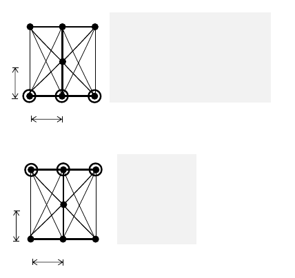
makespan optimal solutions. An example of MAPF

and makespan optimal solution is shown in Figure

1. We note that the standard makespan optimal so-

lution yields makespan suboptimal solution when in-

terpreted as MAPF

Through the straightforward reduction of MAPF

to MAPF

it can be observed that ﬁnding a makespan

optimal solution with continuous time is an NP-hard

problem (Ratner and Warmuth, 1990; Surynek, 2010;

Yu and LaValle, 2015).

2 SOLVING MAPF WITH

CONTINUOUS TIME

We will describe here how to ﬁnd optimal solution

of MAPF

using the conﬂict-based search (CBS)

(Sharon et al., 2015). CBS uses the idea of resolv-

ing conﬂicts lazily; that is, a solution of MAPF in-

1.0

π(a

1 → 1 [0.000, 1.414)

1 → 2 [1.414, 2.414)

2 → 7 [2.414, 4.650)

π(a

3 → 6 [0.000, 2.236)

6 → 5 [2.236, 3.236)

5 → 5 [3.236, 4.650)

μ = 4.650 (MAPF

)

π(a

2 → 4 [0.000, 1.000)

4 → 4 [1.000, 3.236)

4 → 6 [3.236, 4.236)

6 → 6 [4.236, 4.650)

π(a

)

1 → 6

6 → 3

3 → 7

π(a

)

2 → 4

4 → 1

1 → 6

π(a

)

3 → 7

7 → 2

2 → 5

μ = 3 (MAPF)

μ = 6.472 (MAPF

)

ρ.speed = 1.0 ρ.radius = 0.2

MAPF

Figure 1: An example of MAPF

instance on a

[3,1,3]−graph with three agents and its makespan optimal

solution (an optimal solution of the corresponding standard

MAPF is shown too).

stance is not searched against the complete set of

movement constraints. Instead of forbidding all pos-

sible collisions between agents, we start with ini-

tially empty set of collision forbidding constraints that

gradually grows as new conﬂicts appear. CBS that

was originally developed for MAPF, can be modiﬁed

for MAPF

as shown in (Andreychuk et al., 2019a):

let us denote the modiﬁcation CBS

2.1 Conﬂict-Based Search

CBS

is shown using pseudo-code in Algorithm 1.

The high-level of CBS

searches a constraint tree

(CT) using a priority queue (ordered according to the

makespan or other cumulative cost) in the breadth ﬁrst

search manner. CT is a binary tree where each node

N contains a set of collision avoidance constraints

N.constraints - a set of triples (a

,{u,v}, [t

)) for-

bidding occurrence of agent a

in edge {u,v} (or in

vertex u if u = v) at any time between [t

), a solu-

tion N.π - a set of k individual temporal plans, and the

makespan N.µ of the current solution.

The low-level process in CBS

associated with

node N searches temporal plan for individual agent

with respect to set of constraints N.constraints. For

given agent a

, this is the standard single source

shortest path search from α

) to α

) that at

time t must avoid a set of edges (vertices) {{u,v} ∈

E | (a

,{u,v}, [t

)) ∈ N.constraints ∧ t ∈ [t

)}.

Various intelligent single source shortest path algo-

rithms can be applied here such as A*(Hart et al.,

1968).

Algorithm 1: Basic CBS

algorithm for solving

MAPF with continuous time.

1 CBS

(Σ

= (G = (V, E),A,α

,α

,ρ))

2 R.constraints ←

3 R.π ← {shortest temporal plan from α

) to

) | i = 1,2, ..., k}

4 R.µ ← max

i=1

µ(N.π(a

))

5 OPEN ←

6 insert R into OPEN

7 while OPEN 6=

0 do

8 N ← min

(OPEN)

9 remove-Min

(OPEN)

10 collisions ← validate-Plans(N.π)

11 if collisions =

0 then

12 return N.π

13 let (a

,{u,v},[t

)) ×

,{u

},[t

)) ∈ collisions

14 [τ

,τ

) ← [t

) ∩ [t

)

15 for each

(a,{w,z}) ∈ {(a

,{u,v}),(a

,{u

})}

16 N

.constraints ← N.constraints ∪

{(a,{w,z},[τ

,τ

))}

17 N

.π ← N.π

18 update(a, N

.π, N

.con f licts)

19 N

.µ ←

∑

i=1

µ(N

.π(a

))

20 insert N

into OPEN

CBS

stores nodes of CT into priority queue

OPEN sorted according to the ascending makespan.

At each step the algorithm takes node N with the low-

est makespan from OPEN and checks if N.π represent

non-colliding temporal plans. If there is no collision,

the algorithm returns valid MAPF

solution N.π.

Otherwise the search branches by creating a new pair

of nodes in CT - successors of N, each resolving the

collision by diverting one of the colliding agents.

Assume that a collision occurred between agents a

and a

when a

traversed {u, v} during [t

) and

traversed {u

} during [t

). This collision

can be avoided if either agent a

or agent a

does

not occupy {u,v} or {u

} respectively during

) ∩ [t

) = [τ

,τ

) or more precisely we can

calculate unsafe time interval for each agent so that

whenever the agent commences the movement during

this time interval the movement will result in a colli-

sion assuming the other agent following its original

plan. These two options correspond to new successor

nodes of N: N

and N

that inherit set of conﬂicts

from N as follows: N

.con f licts = N.con f licts

∪{(a

,{u,v}, [τ

,τ

))} and N

.con f licts =

N.con f licts ∪{(a

,{u

},[τ

,τ

))}. N

.π and

.π inherit plans from N.π except those for agent a

and a

respectively that are recalculated with respect

to the new sets of conﬂicts. After this N

and N

are

inserted into OPEN.

Deﬁnition of collisions comes as a parameter to

the algorithm though the implementation of validate-

Plans procedure. We can switch to the less cautious

deﬁnition of collisions that reports a collision after

agents actually overlap their bodies. This can be done

through changing the validate-Plans procedure while

the rest of the algorithm remains the same.

2.2 A Satisﬁability Modulo Theory

(SMT) Approach

A close look at CBS reveals that it operates simi-

larly as problem solving in satisﬁability modulo theo-

ries (SMT) (Boﬁll et al., 2012; Nieuwenhuis, 2010).

The basic use of SMT divides a satisﬁability problem

in some complex theory T into an abstract proposi-

tional part that keeps the Boolean structure of the de-

cision problem and a simpliﬁed decision procedure

DECIDE

that decides fragment of T restricted on

conjunctive formulae. A general T -formula Γ being

decided for satisﬁability is transformed to a proposi-

tional skeleton by replacing its atoms with proposi-

tional variables. The standard SAT-solving procedure

then decides what variables should be assigned TRUE

in order to satisfy the skeleton - these variables tells

what atoms hold in Γ. DECIDE

then checks if the

conjunction of atoms assigned TRUE is valid with re-

spect to axioms of T . If so then the satisfying as-

signment is returned and we are ﬁnished. Otherwise

a conﬂict from DECIDE

(often called a lemma) is

reported back to the SAT solver and the skeleton is

extended with new constraints resolving the conﬂict.

In a more general case, not only new constraints are

added to resolve the conﬂict but also new variables

i.e. atoms can be added to Γ.

The above observation inspired us to the idea to

rephrase CBS

in terms of SMT similarly as it has

been previously done with CBS and its reformula-

tion in SMT suggested in (Surynek, 2019). T will

be represented by a theory with axioms describing

movement rules of MAPF

; a theory we will denote

MAPF

A plan validation procedure known from CBS will

act as DECIDE

MAPF

and will report back a set of

conﬂicts found in the current solution. The propo-

sitional part working with the skeleton will be taken

from existing propositional encodings of the stan-

The formal details of the theory T

MAPF

are not rel-

evant from the algorithmic point of view so we will omit

them here. Nevertheless let us note that the signature of

MAPF

consists of non-logical symbols describing agents’

positions at a time such as at(a,u,t) - agent a at vertex u at

time t.

dard MAPF such as the MDD-SAT (Surynek et al.,

2016) provided that constraints forbidding conﬂicts

between agents will be omitted (at the beginning). In

other words, we only preserve constraints ensuring

that propositional assignments form proper paths for

agents but each agent is treated as if it is alone in the

instance (we only forbid agents to jump but we ignore

collisions between them).

2.3 Decision Variable Generation

MDD-SAT introduces decision variables X

) and

u,v

) for discrete time-steps t ∈ {0, 1,2,...} de-

scribing occurrence of agent a

in v or the traversal

of edge {u,v} by a

at time-step t. We refer the reader

to (Surynek et al., 2016) for the details of how to en-

code constraints of top of these variables. As an ex-

ample we show here a constraint stating that if agent

appears in vertex u at time step t then it has to leave

through exactly one edge connected to u or wait in u.

) ⇒

v | {u,v}∈E

u,v

) ∨ E

u,u

), (1)

∑

v | {u,v}∈E

u,v

) + E

u,u

) ≤ 1 (2)

Vertex collisions expressed for example by the fol-

lowing constraint are omitted when the encoding is

being built lazily in the SMT-style. The constraint

says that in vertex v and time step t there is at most

one agent.

∑

∈A | v∈V

) ≤ 1 (3)

A signiﬁcant difﬁculty in MAPF

is that we need

decision variables with respect to continuous time.

Fortunately we do not need a variable for any possible

time but only for important moments.

If for example the duration of a conﬂict in neigh-

bor v of u is [t

) and agent a

residing in u at t ≥ t

wants to enter v then the earliest time a

can do so is

since before it would conﬂict in v (according to the

above deﬁnition of collisions). On the other hand if

does not want to waste time (let us note that we

search for a makespan optimal solution), then waiting

longer than t

is not desirable. Hence we only need

to introduce decision variable E

u,v

) to reﬂect the

situation.

Generally, when having a set of conﬂicts we need

to generate decision variables representing occur-

rence of agents in vertices and edges of the graph at

important moments with respect to the set of conﬂicts.

The process of decision variable generation is for-

mally described as Algorithm 2. It performs breadth-

ﬁrst search (BFS) on G using two types of actions:

Algorithm 2: Generation of decision variables in

the SMT-based algorithm for MAPF

solving.

1 generate-Decisions

(Σ

= (G = (V, E),A,α

,α

,ρ), a

, con f licts,

max

)

2 VAR ←

3 for each a ∈ A do

4 OPEN ←

5 insert (α

(a),0) into OPEN

6 VAR ← VAR ∪ {X

(a)

(a)}

7 while OPEN 6=

0 do

8 (u,t) ← min

(OPEN)

9 remove-Min

(OPEN)

10 if t ≤ µ

max

then

11 for each v such that {u,v} ∈ E do

12 ∆t ← dist(u, v)/v

13 insert (v,t + ∆t) into OPEN

14 VAR ←

VAR ∪{E

u,v

(a),X

t+∆t

(a)}

15 for each v such that

{u,v} ∈ E ∪ {u,u} do

16 for each (a,{u, v}, [t

)) ∈

con f licts do

17 if t

> t then

18 insert (u,t

) into

OPEN

19 VAR ←

VAR ∪{X

(a)}

20 return VAR

edge traversals and waiting. The edge traversal is the

standard operation from BFS. Waiting is performed

for every relevant period of time with respect to the

end-times in the set of conﬂicts of neighboring ver-

tices.

As a result each conﬂict during variable genera-

tion through BFS is treated as both present and absent

which in effect generates all possible important mo-

ments.

Procedure generate-Decision generates decision

variables that correspond to actions started on or be-

fore speciﬁed limit µ

max

. For example variables cor-

responding to edge traversal started at t < µ

max

and

ﬁnished as t

> µ

max

are included (line 10). Variables

corresponding to times greater than µ

max

enable de-

termining what should be the next relevant makespan

limit to test (see the high-level algorithm for details

how the makespan limit is used). Assume having a

decision node corresponding to vertex u at time t at

hand. The procedure ﬁrst adds decision variables cor-

responding to edge traversals from u to neighbors de-

noted v (lines 11-14). Then all possible relevant wait-

ing actions in u with respect to its neighbors v are gen-

erated. Notice that waiting with respect to conﬂicts in

u are treated as well.

2.4 Eliminating Branching in CBS by

Disjunctive Reﬁnements

The SMT-based algorithm itself is divided into two

procedures: SMT-CBS

representing the main loop

and SMT-CBS-Fixed

solving the input MAPF

for

a ﬁxed maximum makespan µ. The major difference

from the standard CBS is that there is no branching

at the high-level. The set of conﬂicts is iteratively

extended during the entire execution of the algorithm

whenever a collision is detected.

Procedures encode-Basic and augment-Basic

build formula F (µ) over the decision variables gener-

ated using the aforementioned procedure. The encod-

ing is inspired by the MDD-SAT approach but ignores

collisions between agents. That is, F (µ) constitutes

an incomplete model for a given input Σ

: Σ

is solv-

able within makespan µ then F (µ) is satisﬁable.

Conﬂicts are resolved by adding disjunctive con-

straints (lines 13-15 in Algorithm 4). The collision is

avoided in the same way as in the original CBS that is

one of the colliding agent is diverted from performing

the action leading to the collision. Consider for ex-

ample a collision on two edges between agents a

and

as follows: a

traversed {u, v} during [t

) and a

traversed {u

} during [t

These two movements correspond to decision

variables E

u,v

) and E

) hence elimination of

the collision caused by these two movements can be

expressed as the following disjunction: ¬E

u,v

) ∨

¬E

). At the level of propositional formula

there is no information about the semantics of a con-

ﬂict happening in the continuous space; we only have

information in the form of above disjunctive reﬁne-

ments. The disjunctive reﬁnements are propagated at

the propositional level from DECIDE

MAPF

that ver-

iﬁes solutions of incomplete propositional models.

The set of pairs of collected disjunctive conﬂicts

is propagated across entire execution of the algorithm

(line 16 in Algorithm 4).

Algorithm 3 shows the main loop of SMT-CBS

The algorithm checks if there is a solution for given

MAPF

of makespan µ. The algorithm starts at

the lower bound for µ that is obtained as the duration

of the longest temporal plan from individual temporal

plans ignoring other agents (lines 3-4).

Then µ is iteratively increased in the main loop

(lines 5-9). The algorithm relies on the fact that the

solvability of MAPF

w.r.t. cumulative objective like

the makespan behaves as a non decreasing monotonic

function. Hence trying increasing makespans eventu-

Algorithm 3: High-level of the SMT-based MAPF

solving.

1 SMT-CBS

(Σ

= (G = (V, E),A,α

,α

,ρ))

2 con f licts ←

3 π ← {π

∗

) a shortest temporal plan from

) to α

) | i = 1,2, ..., k}

4 µ ← max

i=1

µ(π(a

))

5 while TRUE do

6 (π,con f licts, µ

) ←

SMT-CBS-Fixed

(Σ

, con f licts, µ)

7 if π 6= UNSAT then

8 return π

9 µ ← µ

ally leads to ﬁnding the optimal makespan in case of

solvable MAPF

provided we do not skip any rele-

vant makespan µ. The next makespan to try will then

be obtained by taking the current makespan plus the

smallest duration of the continuing movement (line

19 of Algorithm 4). The iterative scheme for trying

larger makespans follows the idea used in MDD-SAT

(Surynek et al., 2016) and before introduced in SAT-

based classical planning algorithm SATPlan (Kautz

and Selman, 1992).

3 EXPERIMENTAL EVALUATION

In this section we present results of the ﬁrst experi-

mentation with SMT-CBS

. We implemented SMT-

CBS

in C++ to evaluate its performance

SMT-CBS

was implemented on top of Glucose

3 SAT solver (Audemard and Simon, 2009) which

ranks among the best SAT solvers according to recent

SAT solver competitions (Balyo et al., 2017). When-

ever possible the SAT solver was consulted in the in-

cremental mode.

It turned out to be important to generate decision

variables in a more advanced way than presented

in Algorithm 2. We need to prune out decisions

from that the goal vertex cannot be reached under

given makespan bound µ

max

. That is whenever we

have a decision (u,t) such that t + ∆t > µ

max

, where

∆t = dist

estimate

(u,α

(a))/v

and dist

estimate

is a

lower bound estimate of the distance between a pair

of vertices, we rule out that decision from further con-

sideration. Moreover we apply a postprocessing step

in which we iteratively remove decisions that have

The complete source codes will be made available

to enable reproducibility of presented results on the au-

thor’s website: http://users.ﬁt.cvut.cz/surynpav/research/

icaart2020.

Algorithm 4: Low-level of the SMT-based MAPF

solving.

1 SMT-CBS-Fixed

(Σ

, con f licts, µ)

2 VAR ← generate-Decisions(Σ

, con f licts, µ)

3 F (µ) ← encode-Basic(VAR, Σ

,con f licts, µ)

4 while TRUE do

5 assignment ← consult-SAT-Solver(F (µ))

6 if assignment 6= UNSAT then

7 π ← extract-Solution(assignment)

8 collisions ← validate-Plans(π)

9 /* DECIDE

MAPF

10 if collisions =

0 then

11 return (π,

0,UNDEF)

12 for each (a

,{u,v},[t

)) ×

,{u

,v;},[t

)) ∈ collisions do

13 Y ← (u = v) ? X

) : E

u,v

)

14 Z ← (u

= v

) ? X

) :

)

15 F (µ) ← F (µ) ∪ {¬Y ∨ ¬Z}

16 [τ

,τ

) ← [t

) ∩ [t

)

17 con f licts ← con f licts ∪

{(a

,{u,v},[τ

,τ

)),

,{u

},[τ

,τ

))}

18 VAR ← generate-Decisions(Σ

con f licts, µ)

19 F (µ) ← augment-

Basic(F (µ), VAR,Σ

,con f licts, µ)

20 µ

← min{t | X

) ∈ VAR ∧t > µ)}

21 return (UNSAT, con f licts, µ

)

no successors. The propositional model is generated

only after this preprocessing.

In addition to SMT-CBS

we re-implemented in

C++ CBS

, currently the only alternative solver for

MAPF

based on own dedicated search (Andreychuk

et al., 2019a). The distinguishing feature of CBS

that at the low-level it uses a more sophisticated sin-

gle source shortest path algorithm that searches for

paths that avoid forbidden intervals, a so-called safe-

interval path planning (SIPP) (Yakovlev and Andrey-

chuk, 2017).

Our implementation of CBS

used the standard

heuristics to improve the performance such as the

preference of resolving cardinal conﬂicts (Boyarski

et al., 2015). Without this heuristic, CBS

usually

exhibited poor performance. In the preliminary tests

with SMT-CBS

, we initially tried to resolve against

single cardinal conﬂict too but eventually it turned out

to be more efﬁcient to resolve against all discovered

conﬂicts (the presented pseudo-code shows this vari-

ant).

All experiments were run on a system with Ryzen 7 3.0

GHz, 16 GB RAM, under Ubuntu Linux 18.

3.1 Benchmarks and Setup

SMT-CBS

and CBS

were tested on synthetic

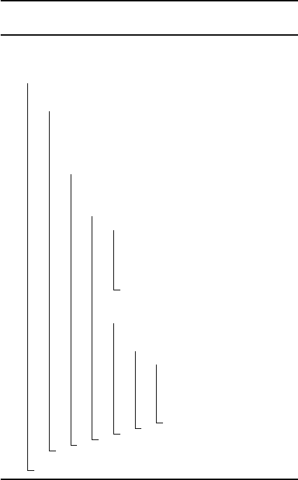
benchmarks consisting of layered graphs, grids, game

maps (Sturtevant, 2012). The layered graph of height

h denoted [l

,...,l

]-graph is a special contruct en-

abling detailed stuty of movements of agents in con-

tinuous space. The layered graph consists of h lay-

ers of vertices placed horizontally above each other in

the 2D plane (see Figure 1 for [3,1,3]-graph). More

precisely the i-th layer is placed horizontally at y = i.

Layers are centered horizontally and the distance be-

tween consecutive points in the layer is 1.0. Size of

all agents was 0.2 in radius.

We measured runtime and the number of deci-

sions/iterations to compare the performance of SMT-

CBS

and CBS

. Small layered graphs consisting of

2 to 5 layers with up to 5 vertices per layer were used

in tests. Three consecutive layers are always fully in-

terconnected by edges. There is no edge across more

than three layers of the graphs. That is in graphs with

more than 3 layers agents cannot go directly to the

goal vertex.

In all tests agents started in the 1-st layer and ﬁn-

ished in the last h-th layer. To obtain instances of var-

ious difﬁculties random permutations of agents in the

starting and goal conﬁgurations were used (the 1-st

layer and h-th layer were fully occupied in the start-

ing and goal conﬁguration respectively). If for in-

stance agents are ordered identically in the starting

and goal conﬁguration with h ≤ 3, then the instance

is relatively easy as it is sufﬁcient that all agents move

simultaneously straight into their goals.

We also used grids of sizes 8 × 8 and 16 × 16

with no obstacles in our tests. Initial and goal con-

ﬁguration of agents have been generated randomly.

In contrast to MAPF benchmarks where grids are 4-

connected we used interconnection with all vertices

in the neighborhood up to certain distance called 2

neighborhood in (Andreychuk et al., 2019a). A simi-

lar setup has been used in game maps (Dragon Age).

The difference here is that the game maps are larger

and contain obstacles.

Ten random instances were generated for individ-

ual graph. The timeout for all tests has been set to 1

minute in layered graphs and small grids and 10 min-

utes for game maps. Results from instances ﬁnished

under this timeout were used to calculate average run-

times.

3.2 Comparison of MAPF

and MAPF

Solving

Part of the results obtained in our experimentation

with layered graphs is shown in Figure 2. The

general observation from our runtime evaluation is

that MAPF

is signiﬁcantly harder than the standard

MAPF. When continuity is ignored, makespan opti-

mal solutions consist of fewer steps. But due to re-

garding all edges to be unit in MAPF, the standard

makespan optimal solutions yield signiﬁcantly worse

continuous makespan (this effect would be further

manifested if we use longer edges).

Average runtime and makespan (μ) on selected layered graphs

Graph

CBS

SMT-CBS

μ MAPF

CBS

μ MAPF

[2,2]

2.78

1.22

2.41

0.01

2.00

[3,1,3]

17.91

2.33

3.65

0.02

2.75

[4,2,2,4]

19.34

4.78

3.80

0.02

2.67

[5,3,1,3,5]

57.23

6.11

6.78

0.03

3.15

[5,3,5,3,5]

19.93

5.39

0.03

3.75

0,00

0,20

0,40

0,60

0,80

1,00

1,20

4 5 6 7 8 9 10 11 12 13 14 15 16 17 18 19 20

Success rate

|V|

Success rate (layered graphs)

CBS-R

SMT-CBS-R

CBS

Figure 2: Comparison of CBS

and SMT-CBS

in terms

of average runtime, makespan, and success rate on layered

graphs. The standard CBS on the corresponding standard

MAPF is shown too (times are in seconds). Makespan is

shown for the case when the instance is interpreted as the

standard MAPF and as MAPF

SMT-CBS

outperforms CBS

on tested in-

stances signiﬁcantly. CBS

reached the timeout

many more times than SMT-CBS

. In the absolute

runtimes, SMT-CBS

is faster by factor of 2 to 10

than CBS

In terms of the number of decisions, SMT-CBS

generates order of magnitudes fewer iterations than

CBS

. This is however expected as SMT-CBS

shrinks the entire search tree into a single branch in

fact. We note that branching within the search space

in case of SMT-CBS

is deferred into the SAT solver

where even more branches may appear.

In case of small grids and large maps (Figures 3,

4 and 5), the difference between CBS

and SMT-

CBS

is generally smaller but still for harder in-

stances SMT-CBS

tends to have better runtime and

success rate. We attribute the smaller difference be-

tween the two algorithms to higher regularity in grids

0,00

0,01

0,10

1,00

10,00

100,00

1 2 3 4 5 6 7 8 9 10 11 12 13 14

Runtime (seconds)

|A|

Average runtime (grid 8x8)

CBS-R SMT-CBS-R CBS

0,00

0,20

0,40

0,60

0,80

1,00

1,20

1 2 3 4 5 6 7 8 9 10 11 12 13 14 15 16

Success rate

|A|

Success rate (grid 8x8)

CBS-R SMT-CBS-R CBS

Figure 3: Comparison of CBS

and SMT-CBS

on 8 × 8

grid with 2

neighborhood (k = 3).

0,00

0,01

0,10

1,00

10,00

100,00

2 4 6 8 10 12 14 16 18 20 22

Runtime (seconds)

|A|

Average runtime (grid 16x16)

CBS-R SMT-CBS-R CBS

0,00

0,20

0,40

0,60

0,80

1,00

1,20

2 4 6 8 10 12 14 16 18 20 22 24

Success rate

|A|

Success rate (grid 16x16)

CBS-R SMT-CBS-R CBS

Figure 4: Comparison of CBS

and SMT-CBS

on 16×16

grid with 2

neighborhood (k = 3).

compared to layered graphs that exhibit higher com-

binatorial difﬁculty.

0,01

0,1

100

1000

2 4 6 8 10 12 14 16 18 20 22

Runtime (seconds)

|A|

Average runtime (Brc202d)

CBS-R SMT-CBS-R CBS

0,01

0,1

100

1000

2 4 6 8 10 12 14 16 18 20 22 24 26 28 30

Runtime (seconds)

|A|

Average runtime (Den520d)

CBS-R SMT-CBS-R CBS

0,01

0,1

100

1000

2 4 6 8 10 12 14 16 18 20 22 24

Runtime (seconds)

|A|

Average runtime (Ost003d)

CBS-R SMT-CBS-R CBS

Figure 5: Comparison of CBS

and SMT-CBS

on game

maps (Dragon Age) with 2

neighborhood (k = 3).

4 DISCUSSION AND

CONCLUSION

We suggested a novel approach for the makespan op-

timal solving of the multi-agent path ﬁnding problem

with continuous time and space based on satisﬁability

modulo theories (SMT). Our approach builds on the

idea of treating constraints lazily as suggested in the

CBS algorithm but instead of branching the search af-

ter encountering a conﬂict we reﬁne the propositional

model with the conﬂict elimination disjunctive con-

straint. The major obstacle in using SMT and propo-

sitional reasoning is that decision variables cannot be

determined in advance straightforwardly in the con-

tinuous case. We hence suggested a novel decision

variable generation approach that enumerates new de-

cisions after discovering new conﬂicts. The proposi-

tional model is iteratively solved by the SAT solver.

We call the novel algorithm SMT-CBS

We compared SMT-CBS

to the only previous

approach for MAPF

that modiﬁes the standard CBS

algorithm (Andreychuk et al., 2019a) and uses dedi-

cated search on a number of benchmarks. The out-

come of our comparison is that SMT-CBS

is faster

than CBS

. We observed the best performance of

SMT-CBS

on layered graphs that constitute com-

binatorially difﬁcult case on a small graph - this is

the case where SMT-CBS

relies mostly on the SAT

solver and less on decision variable generation and

other other high-level mechanisms. We attribute the

better runtime results of SMT-CBS

to more efﬁ-

cient handling of disjunctive conﬂicts in the underly-

ing SAT solver through propagation, clause learning,

and other mechanisms.

Comparison with the standard MAPF version in-

dicate that continuous reasoning is harder to solve but

on the other hand provides more realistic solutions.

Closer analysis of assumptions introduced by the

deﬁnition of MAPF

shows the importance of prede-

ﬁned interconnections between positions in the space.

Currently neither CBS

nor SMT-CBS

can handle

agents that are moving freely in the space along any

trajectory. Such a less restrictive variant of continu-

ous MAPF takes place in completely different search

space and hence searching for a solution would re-

quire different reasoning.

For the future work we assume extending the con-

cept of SMT-based approach for MAPF

with other

cumulative cost functions other than the makespan

such as the sum-of-costs (Sharon et al., 2013b). We

also plan to extend the node generation scheme to di-

rectional agents where we need to add the third di-

mension in addition to space (vertices) and time: di-

rection (angle). We also regard the work in MAPF

as stepping-stone to multi-robot motion planning in

continuous conﬁguration spaces (LaValle, 2006).

ACKNOWLEDGEMENTS

This paper has been supported by the Czech Science

Foundation (application number 19-17966S). The au-

thor would like to thank anonymous reviewers for

their effort to provide valuable comments.

REFERENCES

Andreychuk, A., Yakovlev, K., Atzmon, D., and Stern, R.

(2019a). Multi-agent pathﬁnding (MAPF) with con-

tinuous time. CoRR, abs/1901.05506.

Andreychuk, A., Yakovlev, K. S., Atzmon, D., and Stern,

R. (2019b). Multi-agent pathﬁnding with continuous

time. In Proceedings of the Twenty-Eighth Interna-

tional Joint Conference on Artiﬁcial Intelligence, IJ-

CAI 2019, pages 39–45. ijcai.org.

Audemard, G. and Simon, L. (2009). Predicting learnt

clauses quality in modern SAT solvers. In IJCAI,

pages 399–404.

Balyo, T., Heule, M. J. H., and J

arvisalo, M. (2017). SAT

competition 2016: Recent developments. In AAAI,

pages 5061–5063.

Biere, A., Biere, A., Heule, M., van Maaren, H., and Walsh,

T. (2009). Handbook of Satisﬁability: Volume 185

Frontiers in Artiﬁcial Intelligence and Applications.

IOS Press.

Boﬁll, M., Palah

ı, M., Suy, J., and Villaret, M. (2012). Solv-

ing constraint satisfaction problems with SAT modulo

theories. Constraints, 17(3):273–303.

Boyarski, E., Felner, A., Stern, R., Sharon, G., Tolpin,

D., Betzalel, O., and Shimony, S. (2015). ICBS:

improved conﬂict-based search algorithm for multi-

agent pathﬁnding. In IJCAI, pages 740–746.

ap, M., Nov

ak, P., Vokr

ınek, J., and Pechoucek, M.

(2013). Multi-agent RRT: sampling-based coopera-

tive pathﬁnding. In International conference on Au-

tonomous Agents and Multi-Agent Systems, AAMAS

’13, 2013, pages 1263–1264.

Hart, P. E., Nilsson, N. J., and Raphael, B. (1968). A for-

mal basis for the heuristic determination of minimum

cost paths. IEEE Transactions on Systems Science and

Cybernetics, SSC-4(2):100–107.

onig, W., Kumar, T. K. S., Cohen, L., Ma, H., Xu, H.,

Ayanian, N., and Koenig, S. (2017). Summary: Multi-

agent path ﬁnding with kinematic constraints. In Pro-

ceedings of the Twenty-Sixth International Joint Con-

ference on Artiﬁcial Intelligence, IJCAI 2017, Mel-

bourne, Australia, August 19-25, 2017, pages 4869–

4873.

Janovsky, P., C

ap, M., and Vokr

ınek, J. (2014). Finding co-

ordinated paths for multiple holonomic agents in 2-d

polygonal environment. In International conference

on Autonomous Agents and Multi-Agent Systems, AA-

MAS ’14, 2014, pages 1117–1124.

Kautz, H. A. and Selman, B. (1992). Planning as satisﬁabil-

ity. In Proceedings of the 10th European Conference

on Artiﬁcial Intelligence, ECAI 1992, pages 359–363.

John Wiley and Sons.

Kornhauser, D., Miller, G. L., and Spirakis, P. G. (1984).

Coordinating pebble motion on graphs, the diameter

of permutation groups, and applications. In FOCS,

1984, pages 241–250.

Lam, E., Bodic, P. L., Harabor, D. D., and Stuckey, P. J.

(2019). Branch-and-cut-and-price for multi-agent

pathﬁnding. In Proceedings of the Twenty-Eighth In-

ternational Joint Conference on Artiﬁcial Intelligence,

IJCAI 2019, 2019, pages 1289–1296. ijcai.org.

LaValle, S. M. (2006). Planning algorithms. Cambridge

University Press.

Li, J., Surynek, P., Felner, A., Ma, H., and Koenig, S.

(2019). Multi-agent path ﬁnding for large agents. In

AAAI. AAAI Press.

Ma, H., Koenig, S., Ayanian, N., Cohen, L., H

onig, W.,

Kumar, T. K. S., Uras, T., Xu, H., Tovey, C. A.,

and Sharon, G. (2017). Overview: Generalizations

of multi-agent path ﬁnding to real-world scenarios.

CoRR, abs/1702.05515.

Ma, H., Wagner, G., Felner, A., Li, J., Kumar, T. K. S.,

and Koenig, S. (2018). Multi-agent path ﬁnding with

deadlines. In Proceedings of the Twenty-Seventh In-

ternational Joint Conference on Artiﬁcial Intelligence,

IJCAI 2018, July 13-19, 2018, Stockholm, Sweden.,

pages 417–423.

Nieuwenhuis, R. (2010). SAT modulo theories: Getting the

best of SAT and global constraint ﬁltering. In Prin-

ciples and Practice of Constraint Programming - CP

2010 - 16th International Conference, CP 2010, St.

Andrews, Scotland, UK, September 6-10, 2010. Pro-

ceedings, pages 1–2.

Ratner, D. and Warmuth, M. K. (1990). Nxn puzzle

and related relocation problem. J. Symb. Comput.,

10(2):111–138.

Ryan, M. R. K. (2008). Exploiting subgraph structure in

multi-robot path planning. J. Artif. Intell. Res. (JAIR),

31:497–542.

Sharon, G., Stern, R., Felner, A., and Sturtevant, N.

(2015). Conﬂict-based search for optimal multi-agent

pathﬁnding. Artif. Intell., 219:40–66.

Sharon, G., Stern, R., Felner, A., and Sturtevant, N. R.

(2012). Conﬂict-based search for optimal multi-agent

path ﬁnding. In AAAI.

Sharon, G., Stern, R., Goldenberg, M., and Felner, A.

(2013a). The increasing cost tree search for optimal

multi-agent pathﬁnding. Artif. Intell., 195:470–495.

Sharon, G., Stern, R., Goldenberg, M., and Felner, A.

(2013b). The increasing cost tree search for opti-

mal multi-agent pathﬁnding. Artiﬁcial Intelligence,

195:470–495.

Silver, D. (2005). Cooperative pathﬁnding. In Proceedings

of the First Artiﬁcial Intelligence and Interactive Dig-

ital Entertainment Conference, 2005, pages 117–122.

AAAI Press.

Sturtevant, N. R. (2012). Benchmarks for grid-based

pathﬁnding. Computational Intelligence and AI in

Games, 4(2):144–148.

Surynek, P. (2009). A novel approach to path planning

for multiple robots in bi-connected graphs. In 2009

IEEE International Conference on Robotics and Au-

tomation, ICRA 2009, pages 3613–3619. IEEE.

Surynek, P. (2010). An optimization variant of multi-robot

path planning is intractable. In Proceedings of the

Twenty-Fourth AAAI Conference on Artiﬁcial Intelli-

gence, AAAI 2010. AAAI Press.

Surynek, P. (2012). Towards optimal cooperative path

planning in hard setups through satisﬁability solving.

In PRICAI 2012: Trends in Artiﬁcial Intelligence -

12th Paciﬁc Rim International Conference on Artiﬁ-

cial Intelligence, 2012. Proceedings, volume 7458 of

Lecture Notes in Computer Science, pages 564–576.

Springer.

Surynek, P. (2019). Unifying search-based and

compilation-based approaches to multi-agent path

ﬁnding through satisﬁability modulo theories. In

Proceedings of the Twenty-Eighth International Joint

Conference on Artiﬁcial Intelligence, IJCAI 2019,

2019, pages 1177–1183. ijcai.org.

Surynek, P., Felner, A., Stern, R., and Boyarski, E. (2016).

Efﬁcient SAT approach to multi-agent path ﬁnding un-

der the sum of costs objective. In ECAI, pages 810–

818.

Walker, T. T., Sturtevant, N. R., and Felner, A. (2018). Ex-

tended increasing cost tree search for non-unit cost

domains. In Proceedings of the Twenty-Seventh In-

ternational Joint Conference on Artiﬁcial Intelligence,

IJCAI 2018., pages 534–540.

Wang, K. and Botea, A. (2011). MAPP: a scalable multi-

agent path planning algorithm with tractability and

completeness guarantees. JAIR, 42:55–90.

Yakovlev, K. and Andreychuk, A. (2017). Any-angle

pathﬁnding for multiple agents based on SIPP al-

gorithm. In Proceedings of the Twenty-Seventh In-

ternational Conference on Automated Planning and

Scheduling, ICAPS 2017., page 586.

Yu, J. and LaValle, S. M. (2015). Optimal multi-robot

path planning on graphs: Structure and computational

complexity. CoRR, abs/1507.03289.