New Commercial Representation for Cattle Information Gathering

Jorge Navarro

, Isaac Mart

ın de Diego

, Karen Pr

ıncipe-Aguirre and Mar

ıa Jes

us Algar

Data Science Laboratory, Rey Juan Carlos University, C/ Tulip

an, s/n, 28933, M

ostoles, Spain

Keywords:

Internet of Things, Data Science, Time Series, Cattle Behavior, Representation Information.

Abstract:

As the development of Wireless Sensor Networks improves, new applications of Internet of Things are

emerging in sectors as diverse as military, environmental, health or food. In many of these applications, the

autonomy of the devices is an essential element in order to make reasonable use of them. For the cattle domain,

there is a need for an efﬁcient use of energy by sending few messages that accumulate as much information

as possible. This paper proposes a new strategy for sending summarized information from devices that are

commercially used in cattle to analyze animal behavior. Experiments using 120 different daily time series

related to animal behavior have been performed. The obtained results show that the proposed strategy highly

improves the current operation mode of the equipment.

1 INTRODUCTION

Given the rapid growth that Internet of Things

(IoT) has experienced over recent years through

the development of Wireless Sensor Networks

(WSNs), there is a clear interest from society

in the development of technologies that favor the

communication between people and devices (Tan and

Wang, 2010). This communication allows to control

at any time certain processes that may be key for

some sectors such as military, environmental, health

or home applications among others (Akyildiz et al.,

2002).

Within the wide range of sensors available for

different IoT applications, accelerometers have been

widely used for activity recognition purposes (Ravi

et al., 2005; Brezmes et al., 2009). In the livestock

industry, accelerometers have allowed to record

information about animal status in a myriad of studies

(Martiskainen et al., 2009; Diosdado et al., 2015).

In addition, for processes in which devices are

hardly accessible, it is of crucial importance to

provide long-term autonomies to users of the system

(Duarte-Melo and Liu, 2002). Consequently, there

must be a compromise between the amount of data

sent by WSNs and the expected battery life of

the devices used to gather information within the

system. Animal monitoring in extensive livestock

https://orcid.org/0000-0001-9698-3213

https://orcid.org/0000-0001-5197-2932

https://orcid.org/0000-0002-7539-8522

farming is a clear example of this type of systems.

The more information gathered and sent, the more

energy consumption from wireless devices. However,

reducing the amount of data sent in order to improve

the life of the devices may result in situations in which

the information collected does not faithfully reﬂect

animal behavior.

Hence, there is a need to design information

submissions as efﬁcient as possible, collecting data

that gather the maximum possible knowledge about

animal behavior in each submission. More accurate

representations of animal behavior could improve

real-time problems detection, speed up the reaction

of farmers and reduce the number of potential animal

losses or health issues.

This need is one of the main goals sought by the

Digitanimal project (Digitanimal, 2019). Digitanimal

commercializes several IoT-based devices and

services specially designed to gather and analyze

information about animal behavior in extensive

raising. With the combination of these devices and

services, Digitanimal offers their customers a system

for monitoring animal welfare that can be translated

into an increase in the productivity.

The development of these services and devices

is carried out in collaboration with multiple research

centers and experimental farms within European

projects such as CattleChain (CattleChain, 2019).

As a result of this collaboration, Digitanimal

receives information related to events of interest

that have happened to monitored animals, such

526

Navarro, J., Martín de Diego, I., Príncipe-Aguirre, K. and Algar, M.

New Commercial Representation for Cattle Information Gathering.

DOI: 10.5220/0008978405260534

In Proceedings of the 9th International Conference on Pattern Recognition Applications and Methods (ICPRAM 2020), pages 526-534

ISBN: 978-989-758-397-1; ISSN: 2184-4313

as calvings or heats, through the commercialized

devices. The combination of these sources of

information, collaborations and devices, has allowed

the publication of different studies in the area of IoT

and WSNs (Navarro et al., 2019; P

erez et al., 2019).

In this work a dimensionality reduction technique

and a distance function are combined to analyze

accuracy in the representation of time series. The

major goal is to improve the quality of cattle

information gathering with WSNs.

The remainder of this paper is organized as

follows. Section 2 presents a review of studies

and different techniques used for representation and

comparison of longitudinal data related to animal

behavior as well as a detailed description of the

problem to be solved. In Sections 3 and 4 a new

strategy is proposed for data gathering and evaluated

achieving promising performance improvements. The

results obtained are analyzed and discussed in Section

5. Finally, Section 6 presents the main conclusions of

the study.

2 RELATED WORK

2.1 Background

The analysis of longitudinal data has been a growing

research area during the last years. The wide variety

of sectors in which time series analysis is necessary

has resulted in a large amount of new techniques for

time series representation such as Discrete Fourier

Transformation (Faloutsos et al., 1994), Discrete

Cosine Transformation (Korn et al., 1997) or Discrete

Wavelet Transformation (Chan and Fu, 1999).

The Symbolic Aggregate aproXimation (SAX)

(Lin et al., 2003) is a time series representation

widely used by the community (Lkhagva et al., 2006;

Notaristefano et al., 2013). SAX is a dimensionality

reduction technique that allows the transformation of

numerical time series into a group of symbols or

letters, reducing its size and discretizing its values.

For size reduction, SAX relies on the use of

Piecewise Aggregate Approximation (PAA) (Keogh

et al., 2001) which normalizes, i.e., transform to

mean zero and standard deviation one, and splits

time series into equi-length sections computing the

average value of each one. Once PAA is applied, SAX

discretizes values of the PAA result by mapping the

averages computed to some predeﬁned equiprobable

levels. These levels are identiﬁed with symbols

and calculated through different breakpoints, as seen

in Table 1, that produce equal-sized areas under a

Gaussian curve. This can be done thanks to the

Table 1: Breakpoints (γ) in a Gaussian distribution. From 4

to 8 equiprobable levels (α).

4 5 6 7 8

-0.67 -0.84 -0.97 -1.07 -1.15

0 -0.25 -0.43 -0.57 -0.67

0.67 0.25 0 -0.18 -0.32

—— 0.84 0.43 0.18 0

—— —— 0.97 0.57 0.32

—— —— —— 1.07 0.67

—— —— —— —— 1.15

fact that normalized time series have a Gaussian

distribution (Larsen et al., 1986). SAX offers multiple

advantages against other time series representation

techniques such as dimensionality reduction or lower

bounding of the true distance between the represented

and the original time series (Lin et al., 2003).

Besides time series representation, measuring

distances between time series has also been of

relevance for the scientiﬁc community. Thus,

different similarity metrics and distances have been

proposed like Euclidean distance (Faloutsos et al.,

1994), Dynamic Time Warping (Berndt and Clifford,

1994), Longest Common Subsequence (Vlachos

et al., 2002) or Edit Distance with Real Penalty (Chen

and Ng, 2004).

2.2 Problem Description

Digitanimal commercializes several IoT devices

specially designed to analyze animal behavior. This

work is based on the use of two kind of these devices:

Digitanimal’s core product and a prototype developed

for research purposes. The main aim of the presented

work is to improve the quality of the information sent

by the commercial product through the data gathered

with the research prototype.

The core product of Digitanimal is a collar (see

Figure 1) equipped with a GPS system, a surface

temperature sensor and a 3-axis accelerometer. This

device, placed on the neck of the animal, sends a

message with information captured by its sensors to

the servers of the company, at a ﬁxed time rate of 30

minutes.

The message sending is realized through an IoT-

based communication technology, Sigfox (Sigfox,

2019). This technology introduces important

restrictions regarding the amount of information to

be sent: 12 bytes per message at most and no more

than 140 messages per day or a message every 11

minutes. Currently, the 12 bytes are distributed in the

New Commercial Representation for Cattle Information Gathering

527

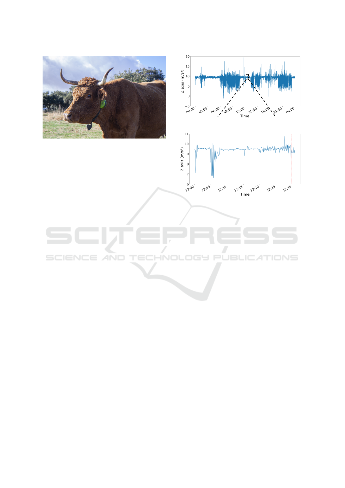
Figure 1: Digitanimal collar placed on an animal.

following way: 42 bits for GPS coordinates, 6 bits

for temperature and 48 bits for accelerometer data (16

bits per axis).

A time rate of 30 minutes allows to ensure that

collars have a battery life for over a year without

the need of replacement. This is one of the main

competitive advantages of Digitanimal and, thus,

this study has not contemplated the possibility of

reducing this rate. Besides, Digitanimal considers 30

minutes as an appropriate time rate for monitoring

animal behavior through one-off GPS and surface

temperature measurements. For this reason, the way

GPS and temperature sensors information is sent has

neither been part of this study.

The gathering of accelerometer information is

carried out differently than the GPS and surface

temperature. Several measurements are taken in a

time window of 30 seconds for each of its axis instead

of just one measurement. Then, average (AVG),

standard deviation (SD) and maximum excursion

(EX) variables are computed from the recorded

measurements. Hence, is essential to increase the

amount of information captured by the accelerometer

within the 30 minutes between each sent message,

taking into account that Digitanimal considers the

AVG variable of greater importance than SD or EX.

On the other hand, the prototype developed

by Digitanimal is a continuous measurement (CM)

device similar to the commercial one. The main

difference between them is that the CM device

only incorporates the accelerometer and it records

information in another way. Every 5 seconds, this

device stores the current position of the accelerometer

in a memory card that is recovered once the data

collection is completed. This device is placed on the

neck of the animal and uses the same green casing as

the commercial one.

Figure 2 shows a representation of the scarce

amount of data captured by commercial devices every

(a) 24 hours of animal activity.

(b) Commercial data recording.

Figure 2: Commercial information gathering in a 30

minutes time window.

time window of 30 minutes. In Figure 2a, animal

movement in the Z axis over 24 hours is represented

in blue. In Figure 2b, a time window of 30 minutes

is enlarged for displaying through red lines the time

while the accelerometer reads the status of the device.

Therefore, the previous 29 minutes and 30 seconds

animal behavior cannot be analyzed, being this issue

the major cause of this study.

Therefore, the main goal of this study is to

improve the quality of the information collected

by the accelerometers of Digitanimal commercial

devices respecting the constraints imposed by Sigfox

technology and the expected battery life. For this

purpose, a new strategy is deﬁned to represent the

time series obtained from CM devices with the

highest possible accuracy.

3 METHODOLOGY

In order to achieve the improvement in the

representation of accelerometer time series sought in

this study, a solution based in SAX is proposed and

evaluated against the current operation mode of the

devices. In this section, the proposed as well as the

commercial solutions are explained in detail.

The main idea behind the evaluation of all

the solutions is based on the assumption that data

ICPRAM 2020 - 9th International Conference on Pattern Recognition Applications and Methods

528

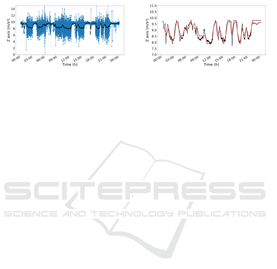
Figure 3: Application of exponential smoothing to the

continuous measurement signal.

collected through CM devices is a close enough

approximation to the real animal behavior. However,

prior to applying any solution to the CM data, it is

necessary to reduce its noise.

Figure 3 shows the application of an exponential

smoothing to the raw CM signal. The transformed

signal is represented through the black curve while

the blue one is the raw data.

3.1 Commercial Solution

With the current commercial solution (CS), the device

turns on automatically every 30 minutes and reads its

status through its sensors. Firstly, the GPS position

and surface temperature are stored to be included

in the ﬁnal message. Then, the accelerometer

takes several measurements of its position during a

time window of 30 seconds at a time rate of 100

milliseconds.

These 300 measurements are used to compute the

AVG, SD and EX variables of the signal within those

30 seconds after applying a low-pass ﬁlter. Finally,

all these values are sent in a message to the servers

of the company using the following distribution of

bits per variable: 6 bits for AVG, 6 bits for SD and

4 bits for EX. As only one measurement is sent per

message, each amount of bits can be used to codify

the information in different possible values following

the relation stated in Equation 1.

Possiblevalues = 2

Number o f bits

(1)

Therefore, this bits distribution means that each

variable (AVG, SD and EX) is discretized in 64, 64

and 16 different possible values, respectively. These

values are computed in an equidistant way within a

range from -2g to 2g, being g the gravity acceleration.

Figure 4 shows the AVG variable of a commercial

signal constructed from the smoothed CM signal. The

red curve represents the commercial one while the

smoothed CM signal is represented in black color.

Each value of the commercial signal is computed

Figure 4: Commercial signal representation for 24 hours.

through the average value of measurements within a

time window of 30 seconds. Therefore, each one of

these values is the average of 6 CM values.

3.2 Proposed Solution

The proposed solution, SAX solution (SS), is

an approach based in the representation technique

explained in Section 2. This solution takes into

account the constraints introduced by Sigfox in order

to deﬁne different possible parameter combinations

of number of levels and equi-length sections for

each variable maintaining the current bit distribution

adopted by Digitanimal. For each combination of

parameters, the amount of available bits will limit

the possible number of levels and sections. Besides

this limitation in the amount of bits per axis and

variable, this study does not consider combinations of

two levels as they reduce excessively the information

sent.

Hence, this solution independently determines

different parameter combinations for the

representation of the AVG, the SD and the EX

variables. As a result, 18 different possible

combinations of levels and sections for each axis are

evaluated. In this work, α and β stand for the levels

and sections of the SS representation. Table 2 shows

some of the ﬁnal possible combinations considered

(for a full view of these combinations see Appendix).

Once deﬁned all the possible combinations, the

ﬁrst step of the solution is the determination of the α

levels. Then, two different approaches are considered

for their computation: equiprobable and equidistance

levels. The normalization of the smoothed CM signal

is required for the division in equiprobable levels. On

the contrary, equidistance levels are computed in the

same way as in the CS.

In the next step, β values are computed within

time windows of 30 minutes. These values are

computed through the mean, standard deviation or

maximum excursion depending on the variable to be

constructed. Then, each β value is mapped to α

New Commercial Representation for Cattle Information Gathering

529

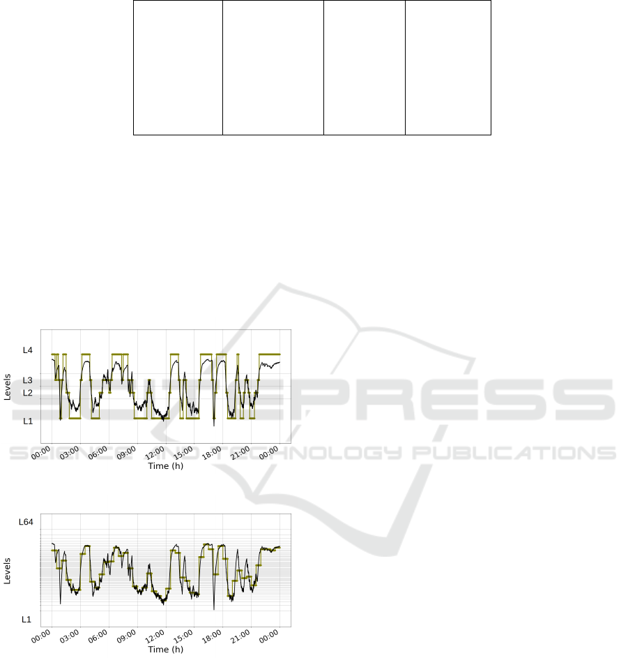
Table 2: SAX Solution (SS) combinations of levels (α) and sections (β) for average (AVG), standard deviation (SD) and

maximum excursion (EX) variables.

Combination AV G

AV G

64 1 4 3 4 2

64 1 4 3 16 1

64 1 8 2 4 2

64 1 8 2 16 1

64 1 64 1 4 2

64 1 64 1 16 1

levels giving shape to the transformed signal. The

deﬁned procedure is applied using every possible

combination speciﬁed in Table 4 as parameters.

Figure 5 serves as an example of the application

of two possible combinations of this procedure to the

CM data for representing the AVG variable. Black

curves represent the smoothed CM signal, while

the green ones are the transformed signal for the

combinations of 4 levels and 3 sections and 64 levels

and 1 section.

(a) α: 4 | β: 3

(b) α: 64 | β: 1

Figure 5: SAX solution applied to two of the possible level

and section combinations.

4 EXPERIMENTAL RESULTS

In order to select the best representation for cattle

information gathering, data from 8 different animals

was captured for 15 days in a row. Hence, a total of

120 different CM daily time series are reconstructed

using each one of the solutions proposed and

compared with the original signal in order to select

the optimal solution.

Next, the strategy for the performance

measurement, different related problems and the

ﬁnal results achieved, are presented.

4.1 Performance Evaluation

For the sake of comparison, each solution is evaluated

following the same performance evaluation method.

The CM signal, splited in time windows of 30

minutes, is used as the reference signal. Thus, the

accuracy of each representation is determined through

its Euclidean distance to the reference signal. For

that matter, as values of the reconstructed signals are

based on some predeﬁned levels, each point of the

CM signal is compared with the middle point of the

corresponding level. Notice that, the CM devices

capture data in time rates of 5 seconds. Thus, every

CM time series contains 48 time windows of 30

minutes made up of 360 points.

To illustrate this process, Figure 6 presents an

example of the error calculation for a 30 minutes

time window between the SS combination of 4 levels

and 3 sections, and the CM signal. For visualization

purposes, the number of points represented for the

CM signal have been reduced to just a 10% of the

original amount. Therefore, just 36 points from

the original 360 has been represented, 12 points per

section. In this case, the error is calculated as the sum

of the Euclidean distances between the CM points and

the SS levels.

The estimation of the representation error implies

two different problems. First, the deﬁnition of a

reference signal to evaluate the reconstruction of SD

and EX for each solution. Next, the determination of

the middle point for the ﬁrst and last levels, in the

proposed representations.

Notice that, in order to evaluate the accuracy of the

AVG variable reconstruction, the original CM values

can be directly used as reference signal. However,

ICPRAM 2020 - 9th International Conference on Pattern Recognition Applications and Methods

530

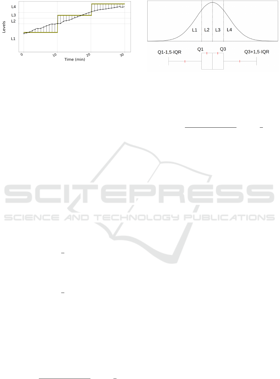
Figure 6: Error calculation within 30 minutes time intervals.

CM signal in black, SS representation in green.

when dealing with SD and EX, new time series are

necessary to compute the Euclidean distance. In this

work, we propose to generate these time series as

follows: SD and EX references are computed per time

windows of 10 minutes from the original CM signal.

Thus, ﬁnal signals of 3 points each 30 minutes (that is

144 points per time series), are used in the evaluation.

The problem of determining the middle point of

ﬁrst and last levels arise because these levels cover

from −∞ to the ﬁrst breakpoint and from the last

breakpoint to +∞. Therefore, choosing their middle

points is not a straightforward decision. To illustrate

the proposed procedure, Figure 7 explains how these

middle points are selected for a SS combination of 4

levels. The 3 breakpoints needed to deﬁne the 4 levels

are represented by vertical lines over the Gaussian

distribution. These breakpoints correspond to the ﬁrst

(Q1) , second (median, Q2) and third (Q3) quartiles

of the Gaussian distribution. Notice that the second

middle point (mp

) is related to Q1 and Q2, and it is

calculated as follows:

(Q2 − Q1) (2)

In the same way, the third middle point (mp

) is

related to the second and third quartiles:

(Q3 − Q2) (3)

First (mp

) and fourth (mp

) middle points are

related to Q1, Q3 and the interquartile range (IQR)

deﬁned as the difference between Q3 and Q1. Thus,

given a boxplot, the middle points for ﬁrst and last

levels are the midpoint between the box and whiskers

given that further values can be considered outliers.

The lower whisker is deﬁned by Q1 − 1.5IQR. Then,

the middle point of the ﬁrst level is obtained as

follows:

= Q1 −

Q1 − (Q1 − 1.5IQR)

= Q1 −

IQR

(4)

Figure 7: Middle point selection for extreme levels.

In the same way, the upper whisker is deﬁned by

Q3 + 1.5IQR. Thus, the middle point of the last level

is obtained as follows:

= Q3 +

(Q3 + 1.5IQR) − Q3

= Q3 +

IQR

(5)

4.2 Final Results

Once the procedure for error calculation has been

deﬁned, the ﬁnal results are computed through the

average error for each one of the 120 available time

series. As the AVG is ﬁxed for the cattle domain

experts as the most relevant variable, a weighted

average is used for the global error calculation. The

ﬁnal error per time series representation is computed

using weights proposed by domain experts as follows:

error = 0.4 · ε

avg

+ 0.3 · ε

(6)

Table 3 presents the error results (per axis) for the

six best SS solutions and for the CS representation

(see the Appendix for a complete table with all the

results). The best overall results are obtained for the

combination SAX

(see Table 4 in the Appendix for

the deﬁnition of this combination). Regarding the CS

solution, error reductions of 31%, 68% and 31% are

achieved for x, y and z axis, respectively, when the

proposed best solution is used.

Figure 8 shows an example of this improvement

for one of the 120 time series. It can be seen that the

SAX solution ﬁts the original CM signal. In addition,

it is possible to detect situations when the CS solution

underﬁt the CM signal. For instance, at time 10 : 30.

In general, the CS solution seems more sensitive to

abrupt changes in the original signal, than the SAX

solution.

New Commercial Representation for Cattle Information Gathering

531

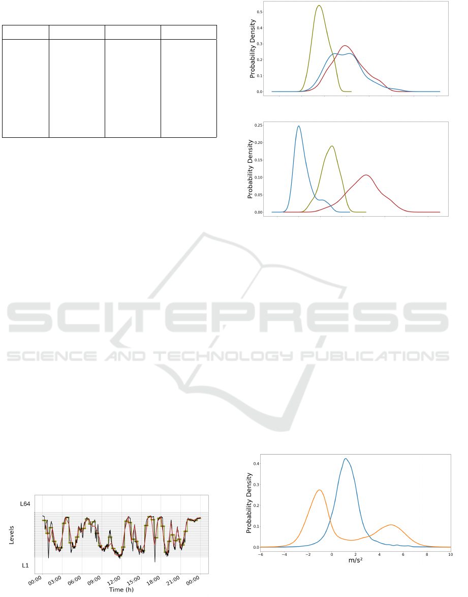
Table 3: Average and standard deviation error rates per axis

for best solutions.

Solution ¯x

error

¯y

error

¯z

error

CS 3.99±0.52 8.72±1.50 3.56±0.41

2.79±0.27 2.88±0.85 2.51±0.26

3.15±0.34 3.12±0.92 2.79±0.33

2.75±0.27 2.82±0.86 2.45±0.27

3.11±0.34 3.06±0.93 2.74±0.34

2.79±0.28 2.84±0.86 2.48±0.28

3.15±0.35 3.09±0.93 2.77±0.36

5 DISCUSSION

The proposed solution for the representation of

cattle information is a valuable alternative to the

current operation mode of devices and, thus, an

improvement in the quality of cattle information

gathering. However, further analysis has been done

revealing that there is still room for improvement.

Figure 9 shows the Probability Density Functions

(PDF) of the errors computed for the AVG variable

in axis X and Y. For the ﬁrst case (X axis), the best

combination (lower errors) is the combination of 64

levels and 1 section for equidistant levels. For the Y

axis, the best combination is the combination of 64

levels and 1 section for equiprobable levels.

This issue is explained through Figure 10. The

blue curve represents the PDF of the measurements

recorded by one of the devices during the 15 days

of the experiment in the X axis, while the orange

one represents the measurements recorded in the

Y axis. Notice that the X axis presents an uni-

modal distribution, that is, a unique type of behavior

is detected. However, the Y axis shows a bi-

modal distribution, that is, two type of behaviors

are presented. This fact is the main reason why

the equiprobable distribution of levels represents in

a more accurate way the animal behavior.

Figure 8: Current and proposed solutions performance

comparison. Black curve represents the original CM signal,

while the red one is the CS and the green one is the SAX

combination.

(a) X axis.

(b) Y axis.

Figure 9: Probability density functions for error rates in

AVG. Red represents the errors for the CS, while green

and blue are the combinations of 64 levels and 1 section

for equidistant and equiprobable levels, respectively.

As in any Data Science project, the proposed

methodology and the obtained results has been

presented and explained to the experts of the domain.

Digitanimal experts’ opinion is that the animal

position with a fewer density seen in Figure 10 for

the Y axis can be associated to grazing animals.

These insights, as others related to different patterns

in animal behavior, can be used to new deﬁnitions

of equiprobable and equidistance levels. Some

animal movements could be explained in a more

accurate way if these levels are validated by experts

considering abnormal behavior situations.

Figure 10: PDF of the X and Y axis, recorded by one of the

devices during the 15 days of the experiment.

ICPRAM 2020 - 9th International Conference on Pattern Recognition Applications and Methods

532

6 CONCLUSIONS

In this work, a novel strategy based in SAX is

proposed to improve the representation of cattle

information gathering through WSNs. As the study

has been promoted within the Digitanimal project,

different insights and requirements from the company

has been considered to deﬁne the solution.

The proposed approach is based on the SAX

representation technique. Different combinations

for the parameters of the SAX representation have

been evaluated, and compared with the current

company solution, through a common procedure for

the estimation of the error. Major improvements have

been achieved.

Besides, the present study is the ﬁrst step towards

the development of higher quality services for the

company. A better accuracy in the representation

of animal behavior could improve real-time problem

detection such as animal calvings or heats.

Next steps and future work will imply different

tasks related to the validation of these results, using

more animals and more days, and development of

new possible strategies. In order to verify the

results achieved in this work, devices programmed

with the proposed solution will be used in future

studies. This task should be done in collaboration

with the company and experimental farms that

allow the new stage of information gathering. On

the other hand, devise of new strategies can be

done expanding the study by introducing different

amount of bits per axis and variables, by using

different representation techniques or even by using

alternative levels deﬁnitions. In this way, the Trend

Segmentation Algorithm (Siordia et al., 2011), the

Trend Feature Symbolic Aggregate approXimation

(Yu et al., 2019) or the Fast Low-cost Online

Semantic Segmentation (Gharghabi et al., 2019)

could be considered.

ACKNOWLEDGEMENTS

Research supported by grants from Madrid

Autonomous Community (Ref: IND2018/TIC-

9665) and European Union’s H2020 Research and

Innovation Program, through the IoF2020 project

(H2020-IoT-2016) under subgrant agreement no.

2282300206-UC010. Special thanks to MISC

International S.L.

REFERENCES

Akyildiz, I. F., Su, W., Sankarasubramaniam, Y., and

Cayirci, E. (2002). Wireless sensor networks: a

survey. Computer networks, 38(4):393–422.

Berndt, D. J. and Clifford, J. (1994). Using dynamic time

warping to ﬁnd patterns in time series. In KDD

workshop, volume 10, pages 359–370. Seattle, WA.

Brezmes, T., Gorricho, J.-L., and Cotrina, J. (2009).

Activity recognition from accelerometer data on a

mobile phone. In International Work-Conference on

Artiﬁcial Neural Networks, pages 796–799. Springer.

CattleChain (2019). Cattlechain, 2019. https://www.

cattlechain.eu/.

Chan, K.-P. and Fu, A. W.-C. (1999). Efﬁcient time

series matching by wavelets. In Proceedings 15th

International Conference on Data Engineering (Cat.

No. 99CB36337), pages 126–133. IEEE.

Chen, L. and Ng, R. (2004). On the marriage of lp-norms

and edit distance. In Proceedings of the Thirtieth

international conference on Very large data bases-

Volume 30, pages 792–803. VLDB Endowment.

Digitanimal (2019). Digitanimal, 2019. https://www.

digitanimal.com/.

Diosdado, J. A. V., Barker, Z. E., Hodges, H. R.,

Amory, J. R., Croft, D. P., Bell, N. J., and Codling,

E. A. (2015). Classiﬁcation of behaviour in housed

dairy cows using an accelerometer-based activity

monitoring system. Animal Biotelemetry, 3(1):15.

Duarte-Melo, E. J. and Liu, M. (2002). Analysis of energy

consumption and lifetime of heterogeneous wireless

sensor networks. In Global Telecommunications

Conference, 2002. GLOBECOM’02. IEEE, volume 1,

pages 21–25. IEEE.

Faloutsos, C., Ranganathan, M., and Manolopoulos, Y.

(1994). Fast subsequence matching in time-series

databases, volume 23. ACM.

Gharghabi, S., Yeh, C.-C. M., Ding, Y., Ding, W., Hibbing,

P., LaMunion, S., Kaplan, A., Crouter, S. E., and

Keogh, E. (2019). Domain agnostic online semantic

segmentation for multi-dimensional time series. Data

mining and knowledge discovery, 33(1):96–130.

Keogh, E., Chakrabarti, K., Pazzani, M., and Mehrotra, S.

(2001). Dimensionality reduction for fast similarity

search in large time series databases. Knowledge and

information Systems, 3(3):263–286.

Korn, F., Jagadish, H. V., and Faloutsos, C. (1997).

Efﬁciently supporting ad hoc queries in large datasets

of time sequences. In Acm Sigmod Record, volume 26,

pages 289–300. ACM.

Larsen, R. J., Marx, M. L., et al. (1986). An introduction to

mathematical statistics and its applications, volume 2.

Prentice-Hall Englewood Cliffs, NJ.

Lin, J., Keogh, E., Lonardi, S., and Chiu, B. (2003).

A symbolic representation of time series, with

implications for streaming algorithms. In Proceedings

of the 8th ACM SIGMOD workshop on Research

issues in data mining and knowledge discovery, pages

2–11. ACM.

New Commercial Representation for Cattle Information Gathering

533

Lkhagva, B., Suzuki, Y., and Kawagoe, K. (2006).

Extended sax: Extension of symbolic aggregate

approximation for ﬁnancial time series data

representation. DEWS2006 4A-i8, 7.

Martiskainen, P., J

arvinen, M., Sk

on, J.-P., Tiirikainen,

J., Kolehmainen, M., and Mononen, J. (2009).

Cow behaviour pattern recognition using a three-

dimensional accelerometer and support vector

machines. Applied animal behaviour science,

119(1-2):32–38.

Navarro, J., Diego, I. M. d., Fern

andez-Isabel, A.,

and Ortega, F. (2019). Fusion of gps and

accelerometer information for anomalous trajectories

detection. In Proceedings of the 2019 the 5th

International Conference on e-Society, e-Learning

and e-Technologies, pages 52–57. ACM.

Notaristefano, A., Chicco, G., and Piglione, F. (2013). Data

size reduction with symbolic aggregate approximation

for electrical load pattern grouping. IET Generation,

Transmission & Distribution, 7(2):108–117.

erez, P. C., Ortega, F., Garc

ıa, J. N., and Diego, I. M. d.

(2019). Combining machine learning and symbolic

representation of time series for classiﬁcation of

behavioural patterns. In Proceedings of the 2019 the

5th International Conference on e-Society, e-Learning

and e-Technologies, pages 93–97. ACM.

Ravi, N., Dandekar, N., Mysore, P., and Littman, M. L.

(2005). Activity recognition from accelerometer data.

In Aaai, volume 5, pages 1541–1546.

Sigfox (2019). Sigfox, 2019. https://www.sigfox.com/.

Siordia, O. S., de Diego, I. M., Conde, C., and

Cabello, E. (2011). Combining trafﬁc safety

knowledge for driving risk detection. In 2011

14th International IEEE Conference on Intelligent

Transportation Systems (ITSC), pages 564–569.

IEEE.

Tan, L. and Wang, N. (2010). Future internet: The internet

of things. In 2010 3rd international conference

on advanced computer theory and engineering

(ICACTE), volume 5, pages V5–376. IEEE.

Vlachos, M., Kollios, G., and Gunopulos, D. (2002).

Discovering similar multidimensional trajectories. In

Proceedings 18th international conference on data

engineering, pages 673–684. IEEE.

Yu, Y., Zhu, Y., Wan, D., Zhao, Q., and Liu, H. (2019).

A novel trend symbolic aggregate approximation for

time series. arXiv preprint arXiv:1905.00421.

APPENDIX

Table 4: SAX Solution (SS) combinations of levels (α) and

sections (β) for AVG, SD and EX variables.

Comb. AV G

AV G

4 3 4 3 4 2

4 3 4 3 16 1

4 3 8 2 4 2

4 3 8 2 16 1

4 3 64 1 4 2

4 3 64 1 16 1

8 2 4 3 4 2

8 2 4 3 16 1

8 2 8 2 4 2

8 2 8 2 16 1

8 2 64 1 4 2

8 2 64 1 16 1

64 1 4 3 4 2

64 1 4 3 16 1

64 1 8 2 4 2

64 1 8 2 16 1

64 1 64 1 4 2

64 1 64 1 16 1

Table 5: Average and standard deviation error rates per axis.

Solution ¯x

error

¯y

error

¯z

error

CS 4.00±0.52 8.72±1.50 3.56±0.41

61.34±8.53 4.06±0.37 6.85±2.78

61.70±8.52 4.31±0.40 7.13±2.79

61.31±8.53 4.01±0.37 6.80±2.78

61.67±8.52 4.25±0.41 7.08±2.80

61.35±8.53 4.03±0.37 6.82±2.79

61.71±8.52 4.27±0.41 7.11±2.81

14.55±3.33 4.27±1.12 6.84±2.76

14.91±3.34 4.52±1.14 7.12±2.77

14.51±3.34 4.22±1.12 6.79±2.76

14.87±3.34 4.46±1.14 7.07±2.78

14.55±3.34 4.24±1.13 6.81±2.77

14.91±3.34 4.48±1.15 7.10±2.78

2.79±0.27 2.88±0.85 2.51±0.26

3.15±0.34 3.12±0.92 2.79±0.33

2.75±0.27 2.82±0.86 2.45±0.27

3.11±0.34 3.06±0.93 2.74±0.34

2.79±0.28 2.84±0.86 2.48±0.28

3.15±0.35 3.09±0.93 2.77±0.36

ICPRAM 2020 - 9th International Conference on Pattern Recognition Applications and Methods

534