
Coarse to Fine Vertebrae Localization and Segmentation
with SpatialConfiguration-Net and U-Net
Christian Payer
1,2 a
, Darko
ˇ
Stern
1,2 b
, Horst Bischof
2 c
and Martin Urschler
1,3 d
1
Ludwig Boltzmann Institute for Clinical Forensic Imaging, Graz, Austria
2
Institute of Computer Graphics and Vision, Graz University of Technology, Graz, Austria
3
School of Computer Science, The University of Auckland, Auckland, New Zealand
Keywords:
Vertebrae Localization, Vertebrae Segmentation, SpatialConfiguration-Net, U-Net, VerSe 2019 Challenge.
Abstract:
Localization and segmentation of vertebral bodies from spine CT volumes are crucial for pathological diagno-
sis, surgical planning, and postoperative assessment. However, fully automatic analysis of spine CT volumes
is difficult due to the anatomical variation of pathologies, noise caused by screws and implants, and the large
range of different field-of-views. We propose a fully automatic coarse to fine approach for vertebrae localiza-
tion and segmentation based on fully convolutional CNNs. In a three-step approach, at first, a U-Net localizes
the rough position of the spine. Then, the SpatialConfiguration-Net performs vertebrae localization and identi-
fication using heatmap regression. Finally, a U-Net performs binary segmentation of each identified vertebrae
in a high resolution, before merging the individual predictions into the resulting multi-label vertebrae segmen-
tation. The evaluation shows top performance of our approach, ranking first place and winning the MICCAI
2019 Large Scale Vertebrae Segmentation Challenge (VerSe 2019).
1 INTRODUCTION
Localization and segmentation of vertebral bodies
from spinal CT volumes is a crucial step for many
clinical applications involving the spine, e.g., patho-
logical diagnosis (Forsberg et al., 2013), surgical
planning (Knez et al., 2016), and postoperative as-
sessment (Amato et al., 2010). Due to the highly
repetitive structure of vertebrae, large variation in the
appearance of different pathologies including frac-
tures and implants, as well as different field-of-views,
most methods for localizing and segmenting vertebral
bodies are based on machine learning. As both local-
ization and segmentation are difficult tasks on their
own, the majority of proposed methods focus on only
one task.
For the task vertebrae localization, or more gen-
erally anatomical landmark localization, a widely
used way of incorporating global shape informa-
tion is to use statistical shape models (Cootes et al.,
1995). (Lindner et al., 2015) extend upon this strat-
a
https://orcid.org/0000-0002-5558-9495
b
https://orcid.org/0000-0003-3449-5497
c
https://orcid.org/0000-0002-9096-6671
d
https://orcid.org/0000-0001-5792-3971
egy by using a constrained local model that itera-
tively refines global landmark configuration on top
of local feature responses generated from random
forests. (Glocker et al., 2012) have combined ran-
dom forests with graphical models based on Markov
random field restricting the responses to only feasi-
ble locations. In addition to extending their method,
(Glocker et al., 2013) have introduced the MICCAI
CSI 2014 Vertebrae Localization and Identification
Challenge dataset, which has been used as a bench-
mark for localizing and identifying vertebrae in spinal
CT volumes. Although a lot of research has focused
on improving landmark localization methods incor-
porating random forests (Ebner et al., 2014; Lindner
et al., 2015; Bromiley et al., 2016; Urschler et al.,
2018), due to the advances of deep learning (Le-
Cun et al., 2015), most recent best-performing meth-
ods for anatomical landmark localization are based
on convolutional neural networks (CNNs). (Chen
et al., 2015) proposed a framework that combines
random forest used for coarse landmark localiza-
tion, a shape model incorporating the information of
neighboring landmarks for refining their positions,
and CNNs for identification of landmarks. How-
ever, their proposed method does not use the full
potential of CNNs, as they are only used for iden-
124
Payer, C., Štern, D., Bischof, H. and Urschler, M.
Coarse to Fine Vertebrae Localization and Segmentation with SpatialConfiguration-Net and U-Net.
DOI: 10.5220/0008975201240133
In Proceedings of the 15th International Joint Conference on Computer Vision, Imaging and Computer Graphics Theory and Applications (VISIGRAPP 2020) - Volume 5: VISAPP, pages
124-133
ISBN: 978-989-758-402-2; ISSN: 2184-4321
Copyright
c
2022 by SCITEPRESS – Science and Technology Publications, Lda. All rights reserved
tification, not for localization. In the related com-
puter vision task human pose estimation, (Toshev and
Szegedy, 2014) introduced CNNs to regress coor-
dinates of landmarks. However, regressing the co-
ordinates directly involves a highly nonlinear map-
ping from input images to point coordinates (Pfis-
ter et al., 2015). Instead of regressing coordinates,
(Tompson et al., 2014) proposed a simpler, image-
to-image mapping based on regressing heatmap im-
ages, which encode the pseudo-probability of a land-
mark being located at a certain pixel position. Us-
ing the heatmap regression framework for anatomical
landmark localization, (Payer et al., 2016) proposed
the SpatialConfiguration-Net (SC-Net) that integrates
spatial information of landmarks directly into an end-
to-end trained, fully-convolutional network. Building
upon (Payer et al., 2016), (Yang et al., 2017) gen-
erate predictions for vertebral landmarks with miss-
ing responses, by incorporating a pre-trained model
of neighboring landmarks into their CNN. Recently,
(Mader et al., 2019) adapted the heatmap regression
networks for predicting more than a hundred land-
marks on a dataset of spinal CT volumes. (Liao
et al., 2018) proposed a three stage method for verte-
brae identification and localization. They pre-train a
network to classify and localize vertebrae simultane-
ously, use the learned weights to generate responses
with a fully convolutional network, and finally re-
move false-positive responses with a bidirectional re-
current neural network. To reduce the amount of in-
formation that needs to be processed, (Sekuboyina
et al., 2018) proposed to project the 3D information
of spine anatomy into 2D sagittal and coronal views,
and solely use these views as input for their 2D CNN
for vertebrae identification and localization. How-
ever, due to this projection, beneficial volumetric in-
formation may be lost. Very recently, (Payer et al.,
2019) improved their volumetric fully convolutional
SC-Net, outperforming other methods on the dataset
of the MICCAI CSI 2014 Vertebrae Localization and
Identification Challenge (Glocker et al., 2013).
For the task vertebrae segmentation, due to the
specific shape of vertebrae, many methods incorpo-
rate models of their shape. Using statistical shape
models, (Klinder et al., 2009) introduce a multi-
stage approach for identifying and segmenting ver-
tebral bodies. (Hammernik et al., 2015) use the
mean shape of a vertebra as initialization for their
convex variational framework. Other methods mod-
eling the vertebra shape include superquadric mod-
els (
ˇ
Stern et al., 2011), models based on game the-
ory (Ibragimov et al., 2014), as well as atlas-based
models (Wang et al., 2016). Similar to vertebrae lo-
calization, recently, machine learning approaches are
Vertebrae
Localization
Spine
Localization
Vertebrae
Segmentation
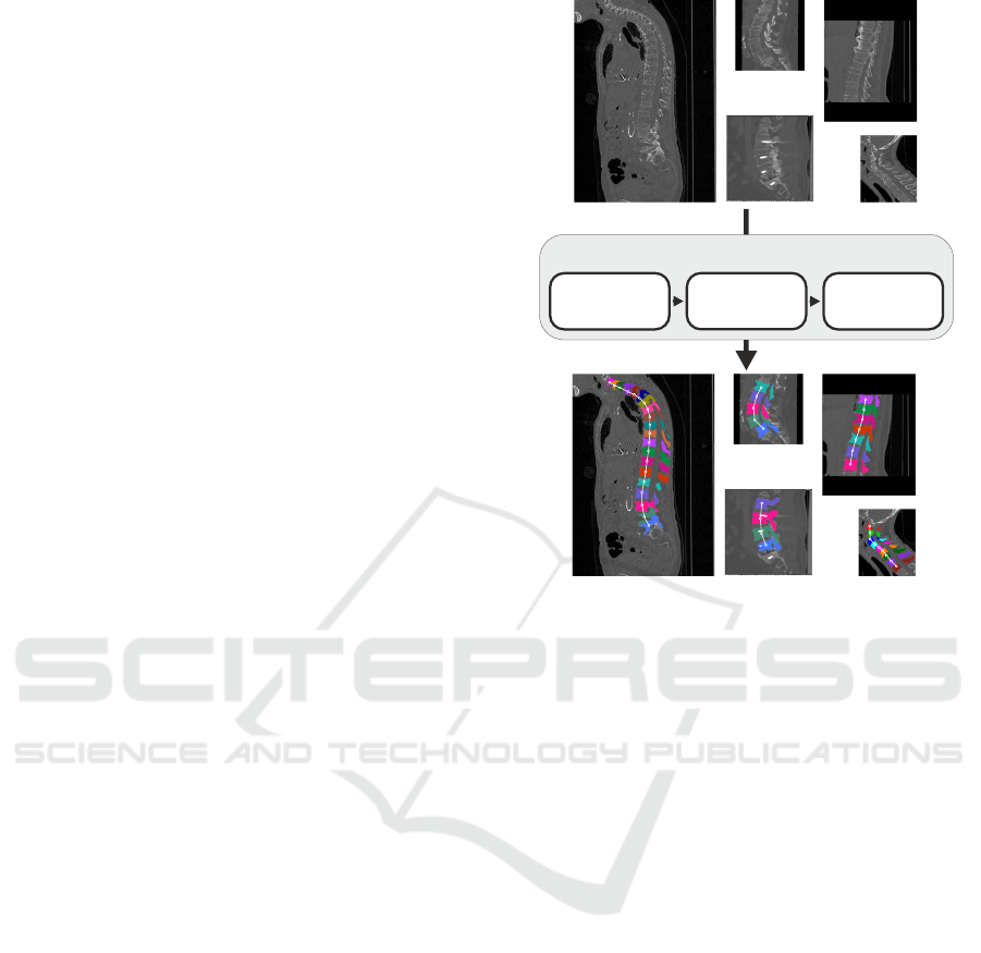
F A, C F
Figure 1: Overview of our proposed coarse to fine fully au-
tomatic vertebrae localization, identification, and segmenta-
tion. The three-step approach works for spine CT volumes
having a large range of different field-of-views, as well as
pathologies.
predominantly used for vertebrae segmentation, due
to the large variation of the appearance and patholo-
gies in clinical CT volumes of the spine. (Chu et al.,
2015) proposed to use random forests for identify-
ing the centroids of vertebral bodies. These centroids
are then used to restrict another random forest that
performs voxelwise labeling and segmentation of the
vertebral body. Coupling shape models with CNNs,
(Korez et al., 2016) use the outputs of a CNN as prob-
ability maps for a deformable surface model to seg-
ment vertebral bodies. Evaluated on the challenging
MICCAI 2016 xVertSeg dataset identifying and seg-
menting lumbar vertebrae, (Sekuboyina et al., 2017)
and (Janssens et al., 2018) use similar two stage ap-
proaches to first localize a bounding box around the
lumbar region, and then to perform a multi-label seg-
mentation of the vertebrae within this region. How-
ever, as the xVertSeg dataset is only used for seg-
menting the five lumbar vertebrae, these methods are
not designed for spinal CT images that have a vary-
ing number of visible vertebrae. A different approach
was introduced by (Lessmann et al., 2019), who use a
single network to use instance segmentation of all ver-
tebrae. By traversing the spinal column with a sliding
window, they propose to segment each vertebra at a
time, while the network incorporates information of
Coarse to Fine Vertebrae Localization and Segmentation with SpatialConfiguration-Net and U-Net
125
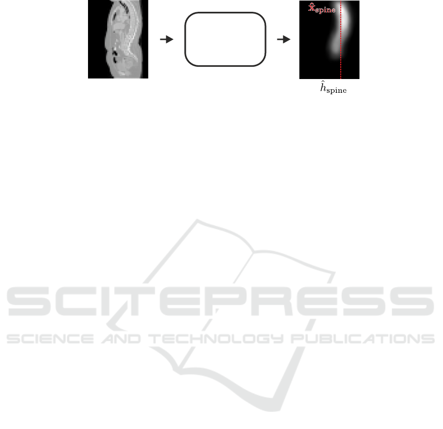
Spine
Localization
U-Net
Network Input
Figure 2: Input volume and the predicted spine heatmap
ˆ
h
spine
of the spine localization network. The predicted coordi-
nate
ˆ
x
spine
is the x and y coordinate of the center of mass of
ˆ
h
spine
.
already segmented vertebrae.
Our main contributions presented in this paper are:
• We developed a coarse to fine fully automatic
method for localization, identification, and seg-
mentation of vertebrae in spine CT volumes. We
first roughly localize the spine, then localize and
identify individual vertebrae, and finally segment
each vertebra in high resolution.
• We tackle the challenging problem of simultane-
ously segmenting and labeling vertebrae in the
presence of highly repetitive structures by doing
the localization and identification step first, and
then doing a binary segmentation of individually
identified vertebrae.
• We perform evaluation and comparison to state-
of-the-art methods on the MICCAI 2019 Large
Scale Vertebrae Segmentation Challenge (VerSe
2019), involving real-world conditions concern-
ing image composition and pathologies. Our pro-
posed method achieves top performance, ranking
first place and winning the VerSe 2019 challenge.
2 METHOD
We perform vertebrae localization and segmentation
in a three-step approach (see Fig. 1). Firstly, due to
the large variation of the field-of-view of the input CT
volumes, a CNN with a coarse input resolution pre-
dicts the approximate location of the spine. Secondly,
another CNN in higher resolution performs multiple
landmark localization and identification of the indi-
vidual vertebra centroids. Lastly, the segmentation
CNN in the highest resolution performs a binary seg-
mentation of each localized vertebra. The results of
the individually segmented vertebrae are then merged
into the final multi-label segmentation.
2.1 Spine Localization
Due to the varying field-of-view, spine CT volumes
often contain lots of background that does not con-
tain useful information, while the spine may not be in
the center of the volume. To ensure that the spine is
centered at the input for the subsequent vertebrae lo-
calization step, as a first step, we predict the approxi-
mate x and y coordinates
ˆ
x
spine
∈ R
2
of the spine. For
localizing
ˆ
x
spine
, we use a variant of the U-Net (Ron-
neberger et al., 2015) to perform heatmap regres-
sion (Tompson et al., 2014; Payer et al., 2016) of
the spinal centerline, i.e., the line passing through
all vertebral centroids. The target heatmap vol-
ume
∗
h
spine
(x;σ
spine
) : R
3
→ R of the spinal center-
line is generated by merging Gaussian heatmaps with
size σ
spine
of all individual vertebrae target coordi-
nates
∗
x
i
into a single volume (see Fig. 2). We use the
L2-loss to minimize the difference between the tar-
get heatmap volume
∗
h
spine
and the predicted heatmap
volume
ˆ
h
spine
(x) : R
3
→ R. The final predicted spine
coordinate
ˆ
x
spine
is the x and y coordinate of the center
of mass of
ˆ
h
spine
.
Our variant of the U-Net is adapted such that it
performs average instead of max pooling and linear
upsampling instead of transposed convolutions. It
uses five levels where each convolution layer has a
kernel size of [3×3×3] and 64 filter outputs. Further-
more, the convolution layers use zero padding such
that the network input and output sizes stay the same.
Before processing a spine CT volume, it is resam-
pled to a uniform voxel spacing of 8 mm and centered
at the network input. The network input resolution is
[64 × 64×128], which allows spine CT volumes with
an extent of up to [512 × 512 × 1024] mm to fit into
the network input. This extent was sufficient for the
network to predict x
spine
for all spine CT volumes of
the evaluated dataset.
VISAPP 2020 - 15th International Conference on Computer Vision Theory and Applications
126
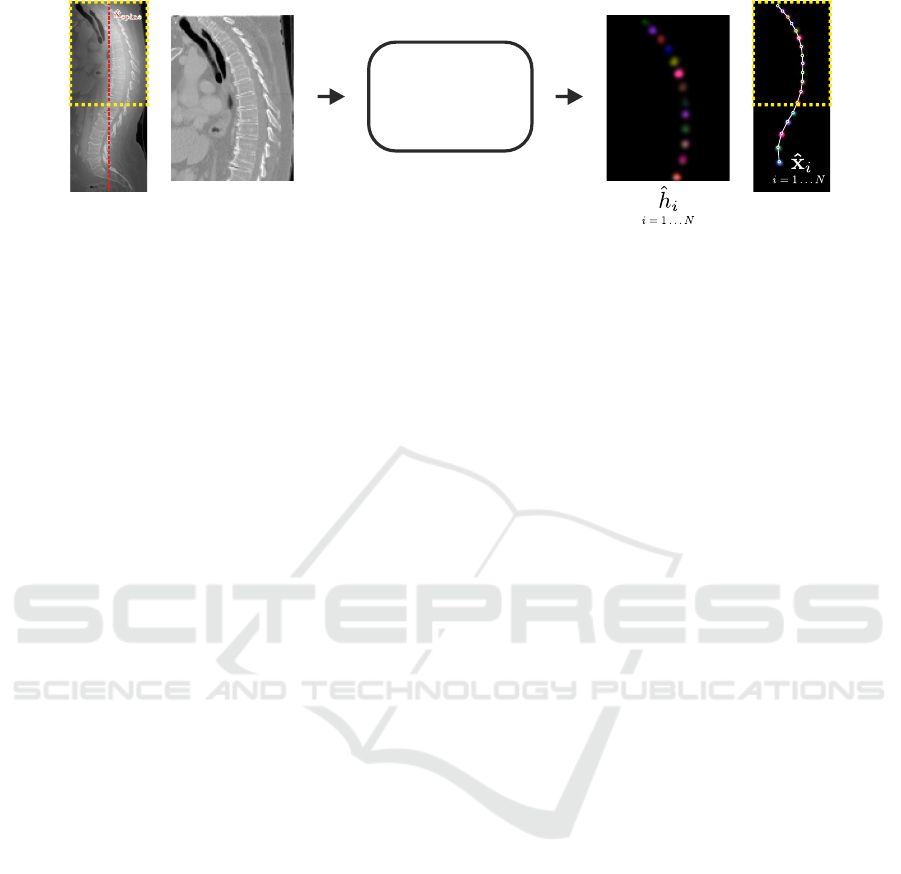
Vertebrae
Localization
SC-Net
Network Input
Figure 3: Input volume and individual heatmap predictions of the vertebrae localization network. The yellow rectangle
indicates that not the whole input volume is processed at once, but overlapping cropped sub-volumes that are centered at
ˆ
x
spine
.
The network predicts simultaneously N heatmaps, i.e., a single heatmap
ˆ
h
i
for each individual vertebrae v
i
. For visualization,
the predicted heatmaps are colored individually and combined into a single image. The final landmark coordinates
ˆ
x
i
are
identified as the longest sequence of local maxima of
ˆ
x
i
that does not violate anatomical constraints.
2.2 Vertebrae Localization
To localize centers of the vertebral bodies, we
use the SpatialConfiguration-Net (SC-Net) proposed
in (Payer et al., 2019). The network effectively com-
bines the local appearance of landmarks with their
spatial configuration. The local appearance part of
the network uses five levels consisting of two convo-
lution layers before downsampling to the lower level,
and two convolution layers after concatenating with
the upsampled lower level. Each convolution layer
uses a leaky ReLU activation function and has a ker-
nel size of [3 ×3×3] and 64 filter outputs. The spatial
configuration part consists of four convolutions with
[7 × 7 × 7] kernels in a row and is processed in one
fourth of the resolution of the local appearance part.
The SC-Net performs heatmap regression of the N
target vertebrae v
i
with i = 1 . . . N, i.e., each target
coordinate
∗
x
i
is represented as a Gaussian heatmap
volume
∗
h
i
(x;σ
i
) : R
3
→ R centered at
∗
x
i
. For N tar-
get vertebrae v
i
, the network predicts simultaneously
all N output heatmap volumes
ˆ
h
i
(x) : R
3
→ R. As loss
function, we use a modified L2-loss function, which
also allows learning of the individual σ
i
values for the
target Gaussian heatmap volumes
∗
h
i
:
L =
N
∑
i=1
∑
x
k
ˆ
h
i
(x) −
∗
h
i
(x;σ
i
)k
2
2
+ αkσ
i
k
2
2
. (1)
For more details of the network architecture and loss
function, we refer to (Payer et al., 2019).
A schematic representation of how the input vol-
umes are processed to predict all heatmaps
ˆ
h
i
is shown
in Fig. 3. Each network input volume is resampled
to have a uniform voxel spacing of 2 mm, while the
network is set up for inputs of size [96 × 96 × 128],
which allows volumes with an extent of [192× 192 ×
256] mm to fit into the network. With this extent,
many images of the dataset do not fit into the net-
work and cannot be processed at once. To narrow the
processed volume to the approximate location of the
spine, we center the network input at the predicted
spine coordinate
ˆ
x
spine
(see Sec. 2.1). Furthermore,
as some spine CT volumes have a larger extent in the
z-axis (i.e., the axis perpendicular to the axial plane)
that would not fit into the network, we process such
volumes the same way as proposed by (Payer et al.,
2019). During training, we crop a subvolume at a ran-
dom position at the z-axis. During inference, we split
the volumes at the z-axis into multiple subvolumes
that overlap for 96 pixels, and process them one after
another. Then, we merge the network predictions of
the overlapping subvolumes by taking the maximum
response over all predictions.
We predict the final landmark coordinates
ˆ
x as fol-
lows: For each predicted heatmap volume, we detect
multiple local heatmap maxima that are above a cer-
tain threshold. Then, we determine the first and last
vertebrae that are visible on the volume by taking the
heatmap with the largest value that is closest to the
volume top or bottom, respectively. We identify the
final predicted landmark sequence by taking the se-
quence that does not violate the following conditions:
consecutive vertebrae may not be closer than 12.5 mm
and farther away than 50 mm, as well as the following
landmark may not be above a previous one.
2.3 Vertebrae Segmentation
For creating the final vertebrae segmentation, we use
a U-Net (Ronneberger et al., 2015) set up for binary
segmentation to separate a vertebra from the back-
ground (see Fig. 4). The final semantic label of a
vertebra is identified through the localization label as
predicted by the vertebrae localization network (see
Sec. 2.2). Hence, we use a single network for all
Coarse to Fine Vertebrae Localization and Segmentation with SpatialConfiguration-Net and U-Net
127

Vertebrae
Segmentation
U-Net
Network Input
Figure 4: Input volume and segmented vertebrae of the spine segmentation network. The yellow rectangle shows the cropped
region around a single vertebrae v
i
and indicates that each localized vertebra
ˆ
x
i
is processed individually. Each individual
vertebra sigmoid prediction
ˆ
l
i
is then transformed and resampled back to the original position. The final multi-label segmen-
tation
ˆ
l
final
is obtained by setting the label at each voxel to the label of
ˆ
l
i
that has the largest response.
vertebrae v
i
, as the network does not need to iden-
tify, which vertebra it is segmenting, but it only needs
to separate each vertebra individually from the back-
ground.
Since each vertebra is segmented independently,
the network needs to know, which vertebra it should
segment in the input volume. Thus, from the whole
spine CT image, we crop the region around the lo-
calized vertebra, such that the vertebra is in the
center of the cropped image. During training, we
use the ground-truth vertebra location
∗
x
i
, while dur-
ing inference, we use the predicted vertebra coordi-
nate
ˆ
x
i
. Additionally, we create an image of a Gaus-
sian heatmap centered at the vertebra coordinate
ˆ
x
i
.
Both the cropped and the heatmap image are used
as an input for the segmentation U-Net. The U-Net
is modified as described in Sec. 2.1. It is set up to
predict a single output volume
ˆ
l
i
(x) : R
3
→ (0, 1),
while the sigmoid cross-entropy loss is minimized
to generate predictions close to the target binary la-
bel volume
∗
l
i
(x) : R
3
→ {0, 1}. The input volumes
are resampled to have a uniform voxel spacing of
1 mm, while the network is set up for inputs of size
[128 × 128 × 96], which allows volumes with an ex-
tent of [128 ×128 × 96] mm.
To create the final multi-label segmentation result,
the individual predictions of the cropped vertebra in-
puts need to be merged. Therefore, the sigmoid out-
put volumes
ˆ
l
i
of each cropped vertebrae i are trans-
formed and resampled back to their position in the
original input volume. Then, for each voxel in the fi-
nal label image
ˆ
l
final
(x) : R
3
→ {0 . . . N}, the predicted
label is set to the label i of the vertebra that has the
largest sigmoid response. If for a pixel no vertebra
prediction
ˆ
l
i
has a response > 0.5, the pixel is set to
be the background.
3 EVALUATION
We evaluate our proposed framework for multi-label
spine localization and segmentation on the dataset of
the VerSe 2019 challenge
1
. The dataset consists of
spine CT volumes of subjects with various patholo-
gies, where every fully visible vertebra from C1 to
L5 is annotated. As some subjects contain the addi-
tional vertebra L6, at maximum N = 25 vertebrae are
annotated. The training set consists of 80 spine CT
volumes with corresponding ground-truth centroids
∗
x
i
and segmentations
∗
l
i
for each vertebra v
i
.
The VerSe 2019 challenge contains two test sets.
The first test set consists of 40 publicly available spine
CT volumes with hidden annotations. The partici-
pants of the challenge had to submit the predictions
on the first test set to the evaluation servers, which
did in turn evaluate and rank the submitted results on
a public leaderboard. The second test set consists of
an additional 40 hidden spine CT volumes. To ob-
tain evaluation results on the second test set, the chal-
lenge participants had to submit a Docker image of
the proposed method that creates the predictions. The
organizers of the challenge then performed an inter-
nal evaluation on the hidden second test set. The final
rank of each participant of the VerSe 2019 challenge
is defined by the performance on the 80 CT volumes
of both test sets and was announced at the workshop
of MICCAI 2019 (Sekuboyina, 2019).
3.1 Implementation Details
Training and testing of the network were done in Ten-
sorflow
2
, while we perform on-the-fly data prepro-
1
https://verse2019.grand-challenge.org/
2
https://www.tensorflow.org/
VISAPP 2020 - 15th International Conference on Computer Vision Theory and Applications
128

Table 1: Results of a three-fold cross-validation on the VerSe 2019 challenge training set consisting of 80 volumes. The table
shows results grouped by cervical, thoracic, and lumbar vertebrae, as well as results for all vertebrae combined.
Vertebrae v
i
PE
i
(in mm)
mean ± SD
ID
i
% (#identified of #total)
Dice
i
mean ± SD
H
i
(in mm)
mean ± SD
Cervical (i = C1 . . . C7) 7.45 ± 8.70 91.07% (102 of 112) 0.91 ± 0.10 5.88 ± 9.50
Thoracic (i = T1 . . . T12) 5.56 ± 6.31 88.99% (388 of 436) 0.93 ± 0.14 6.78 ± 16.67
Lumbar (i = L1 . . . L6) 4.48 ± 2.08 90.45% (284 of 314) 0.96 ± 0.02 6.41 ± 9.05
All (i = C1 . . . L6) 5.71 ± 6.28 89.79% (774 of 862) 0.94 ± 0.11 6.53 ± 13.49
cessing and augmentation using SimpleITK
3
. We per-
formed network and data augmentation hyperparam-
eter evaluation on initial cross-validation experiments
using the training set of the VerSe 2019 challenge.
All networks are trained with a mini-batch size of 1,
while the spine localization network is trained for
20,000 iterations, the vertebrae localization network
for 100,000 iterations, and the vertebrae segmenta-
tion network for 50,000 iterations. For the U-Net we
use the Adam optimizer (Kingma and Ba, 2015) with
a learning rate of 10
−4
, for the SC-Net we use the
Nesterov (Nesterov, 1983) optimizer with a learning
rate of 10
−8
. The spine and vertebrae localization net-
works use L2 weight regularization factor of 5
−4
, the
vertebrae segmentation network uses a factor of 10
−7
.
We set σ
spine
= 3 pixel for the spine localization net-
work; Same as in (Payer et al., 2019), we set α = 100
in (1) for learning the size σ
i
of the target heatmaps
∗
h
i
in the vertebrae localization network.
Due to the different orientations, each CT vol-
ume is transformed into a common orientation for
further processing. Furthermore, to reduce noise on
the input volumes, they are smoothed with a Gaus-
sian kernel with σ = 0.75 mm. To obtain an appro-
priate range of intensity values for neural networks,
each intensity value of the CT volumes is divided
by 2048 and clamped between −1 and 1. For data
augmentation during training, the intensity values are
multiplied randomly with [0.75, 1.25] and shifted by
[−0.25, 0.25]. The images are randomly translated by
[−30, 30] voxels, rotated by [−15
◦
, 15
◦
], and scaled
by [−0.85, 1.15]. We additionally employ elastic de-
formations by randomly moving points on a regular
6×6 pixel grid by 15 pixels and interpolating with 3rd
order B-splines. All augmentation operations sample
randomly from a uniform distribution within the spec-
ified intervals.
Training took ≈ 3:30 h for the spine localization
network, ≈ 28:00 h for the vertebrae localization net-
work, and ≈ 12:00 h for the vertebrae segmentation
network, on an Intel Core i7-4820K workstation with
an NVIDIA Titan V running Arch Linux. The in-
ference time is dependent on the field-of-view and
3
http://www.simpleitk.org/
the number of visible vertebrae on the input CT vol-
ume. On the 40 volumes of the test 1 set of the VerSe
2019 challenge, inference per volume takes on aver-
age ≈ 4:20 m, divided into ≈ 5 s for spine localiza-
tion, ≈ 45 s for vertebrae localization, and ≈ 3:30 m
for vertebrae segmentation.
3.2 Metrics
The localization performance is evaluated with two
commonly used metrics from the literature, describ-
ing localization error in terms of both local accuracy
and robustness towards landmark misidentification.
The first measure, the point-to-point error PE
( j)
i
for
each vertebra i in image j, is defined as the Euclidean
distance between the target coordinate
∗
x
( j)
i
and the
predicted coordinate
ˆ
x
( j)
i
. This allows calculation of
the mean and standard deviation (SD) of the point-to-
point error for all images overall or only a subset of
landmarks. The second measure, the landmark iden-
tification rate ID
i
, is defined as the percentage of cor-
rectly identified landmarks over all landmarks i. As
defined by (Glocker et al., 2013), a predicted land-
mark is correctly identified, if the closest ground-truth
landmark is the correct one, and the distance from
predicted to ground-truth position is less than 20 mm.
The segmentation performance is also evaluated
with two commonly used metrics from the literature.
The first measure is the Dice score Dice
( j)
i
for each
label i in image j, which is defined as twice the car-
dinality of the intersection of ground-truth label
∗
l
( j)
i
and predicted label
ˆ
l
( j)
i
divided by the sum of the car-
dinality of both ground-truth and prediction. The sec-
ond measure is the Hausdorff distance H
( j)
i
between
ground-truth label
∗
l
( j)
i
and predicted label
ˆ
l
( j)
i
for each
label i in image j, which is defined as the greatest of
all the distances from a point in one set to the closest
point in the other set. For both measures, the mean
and standard deviation for all images over all or only
a subset of labels are calculated.
Coarse to Fine Vertebrae Localization and Segmentation with SpatialConfiguration-Net and U-Net
129

Table 2: Results on the overall VerSe 2019 challenge test set, which is comprised of 40 volumes in test 1 set and 40 volumes
in test 2 set. The table lists all methods that submitted valid localizations or segmentations, which allowed the organizers to
calculate the evaluated metrics. The predictions for vertebrae localization and segmentation of test 1 set were generated and
submitted by the participants, while the predictions of test 2 set were generated by the organizers with the submitted Docker
images. The methods are ranked as described in the VerSe 2019 challenge evaluation report (Sekuboyina, 2019). The metrics
show the mean values for all vertebrae of test 1 and test 2 set, respectively. Entries with a ”–” indicate failure of metric
calculation, because of erroneous or missing predictions, or missing Docker images.
Rank Team Score
test 1 set test 2 set
ID
all
PE
all
DSC
all
H
all
ID
all
PE
all
DSC
all
H
all
1
st
christian payer 0.691 95.65 4.27 0.909 6.35 94.25 4.80 0.898 7.34
2
nd
iFLYTEK 0.597 96.94 4.43 0.930 6.39 86.73 7.13 0.837 11.67
3
rd
nlessmann 0.496 89.86 14.12 0.851 8.58 90.42 7.04 0.858 9.01
4
th
huyujin 0.279 – – 0.847 12.79 – – 0.818 29.44
5
th
yangd05 0.216 62.56 18.52 0.767 14.09 67.21 15.82 0.671 28.76
6
th
ZIB 0.215 71.63 11.09 0.670 17.35 73.32 13.61 0.690 19.25
7
th
AlibabaDAMO 0.140 89.82 7.39 0.827 11.22 – – – –
8
th
christoph 0.107 55.80 44.92 0.431 44.27 54.85 19.83 0.464 42.85
9
th
INIT 0.084 84.02 12.40 0.719 24.59 – – – –
10
th
brown 0.022 – – 0.627 35.90 – – – –
11
th
LRDE 0.007 0.01 205.41 0.140 77.48 0.00 1000.00 0.356 64.52
3.3 Results
We evaluated our proposed framework on the
MICCAI VerSe 2019 Grand Challenge. We per-
formed a three-fold cross-validation on the publicly
available training set consisting of 80 annotated vol-
umes to evaluate the individual steps of our proposed
approach, i.e., spine localization, vertebrae localiza-
tion, and vertebrae segmentation. As the purpose of
this cross-validation is to show the performance of the
individual steps, instead of using the predictions of
the previous steps as inputs (i.e.,
ˆ
x
spine
for vertebrae
localization, and
ˆ
x
i
for vertebrae segmentation), the
networks use the ground-truth annotations as inputs
(i.e.,
∗
x
spine
for vertebrae localization, and
∗
x
i
for verte-
brae segmentation).
The results for the three-fold cross-validation of
the individual steps of our approach are as follows:
For spine localization, the PE
spine
mean ± SD is
4.13 ± 8.97 mm. For vertebrae localization and seg-
mentation, Table 1 shows quantitative results for the
cervical, thoracic, and lumbar vertebrae, as well as for
all vertebrae combined.
We participated in the VerSe 2019 challenge at
MICCAI 2019 to evaluate our whole fully automatic
approach and compare the performance to other meth-
ods. For this, we trained the three individual net-
works for spine localization, vertebrae localization,
and vertebrae segmentation on all 80 training images.
We performed inference on the test volumes by us-
ing the predictions from the previous step as inputs
for the next step. We submitted our predictions on
the test 1 set, as well as a Docker image for the or-
ganizers to generate predictions on the hidden test 2
set. Table 2 shows the quantitative results on the test 1
and test 2 sets of methods that submitted valid predic-
tions before the deadlines of the VerSe 2019 challenge
as announced at the challenge workshop at MICCAI
2019 (Sekuboyina, 2019). Our fully automatic ap-
proach ranked first on the combined localization and
segmentation metrics on the overall 80 volumes of
both test sets.
4 DISCUSSION
As announced at the VerSe 2019 workshop at
MICCAI 2019, our method won the VerSe 2019
challenge. Our fully automatic vertebrae localiza-
tion and segmentation ranked first on the 80 volumes
of both test 1 and test 2 set combined, supporting
the proposed three-step approach that combines the
SpatialConfiguration-Net (Payer et al., 2019) and the
U-Net (Ronneberger et al., 2015) in a coarse to fine
manner.
The cross-validation experiments on the 80 anno-
tated training volumes confirm the good performance
of the individual steps of our proposed three-step ap-
proach (see Sec. 3.3 and Table 1). The first stage,
the spine localization, performs well in approximat-
ing the center position of the spine, achieving a point
error PE
spine
of 4.13 mm. Visual inspection showed
only one failure case for a CT volume that is com-
pletely out of the training data distribution. This vol-
ume does not show the spine, but the whole legs. Only
in the top of the volume, a small part of the spine is
VISAPP 2020 - 15th International Conference on Computer Vision Theory and Applications
130

visible, specifically the two vertebrae L4 and L5.
The second stage, the vertebrae localization,
achieves a mean point error PE
all
of 5.71 mm and an
identification rate ID
all
of 89.79% for all vertebrae.
By analyzing the individual predictions for cervical,
thoracic, and lumbar vertebrae, we see differences
among the vertebrae types. As the thoracic vertebrae
are in the middle, being far away from the visible top
or bottom of the spine, it is harder for the network
to distinguish between these vertebrae. This can be
seen in the smaller ID
thoracic
of 88.99%, as compared
to ID
cervical
= 91.07% and ID
lumbar
= 90.45%. How-
ever, having more training data of individual verte-
brae helps the networks for predicting the vertebral
centroids more accurately, which can be seen at the
smaller PE
lumbar
of 4.48 mm (on average ≈ 62 anno-
tations) as compared to PE
thoracic
= 5.56 mm (≈ 36
annotations) and PE
lumbar
= 7.45 mm (≈ 16 annota-
tions per vertebrae).
Having more annotations per vertebrae is also
beneficial for the final third stage, the vertebrae seg-
mentation. Here we can observe that again the lum-
bar vertebrae have the best performance in terms of
Dice score Dice
lumbar
= 0.96, while the Dice score de-
creases with less training data per vertebrae type, i.e.,
Dice
thoracic
= 0.93 and Dice
cervical
= 0.91. However,
for the Hausdorff metric H , we do not see notewor-
thy differences among the vertebrae types. Moreover,
the standard deviations of H are large, which indi-
cates outliers. We think that this is due to noise in the
ground-truth annotation, sometimes containing spu-
riously annotated voxels far off the actual vertebrae
region. Such misannotated isolated pixels are negli-
gible in the Dice score, but lead to large errors and
standard deviations in the Hausdorff metric.
The values on the test sets consisting of 80 vol-
umes in Table 2 demonstrate the overall performance
of our fully automatic, coarse to fine approach. When
compared with the results of the cross-validation, the
localization results improved on both test sets, as can
be seen in both PE
all
= 4.27 mm and PE
all
= 4.80 mm,
as well as ID
all
= 95.65% and ID
all
= 94.25%. This
indicates that the localization network benefits from
more training data (80 CT volumes in the test sets as
compared to ≈ 54 in the cross-validation), especially
due to the large variation and different pathologies in
the dataset.
For the segmentation metrics, the results on the
test sets are slightly worse as compared to the cross-
validation, i.e., Dice
all
= 0.909 and Dice
all
= 0.898, as
well as H
all
= 6.35 mm and H
all
= 7.34 mm. The rea-
son for this performance drop is that the vertebrae seg-
mentation is dependent on the vertebrae localization.
In contrast to the cross-validation, which uses the
ground-truth vertebral centroids
∗
x
i
as input to show
the performance of the segmentation network alone,
the segmentation network that generated results on
the test sets takes the predicted vertebral centroids
ˆ
x
i
as input to show the performance of the whole fully
automatic approach.
When compared to other methods on both test
sets, our method achieves the overall best perfor-
mance. There exists a large gap between our method
and the next best ranking methods in both localiza-
tion and segmentation performance. However, when
looking at the individual test sets, we can see that in
test 1 set the second-best method has a better ID
all
and
Dice
all
as compared to our method, while our method
has a better PE
all
and H
all
. Nevertheless, in test 2 set
the second-best method has a performance drop in all
evaluation metrics, while the results from our method
are stable. The better performance on the hidden test 2
set shows the good generalization capabilities of our
method, enabling it to surpass all other methods and
to win the VerSe 2019 challenge.
5 CONCLUSION
In this paper, we have presented a three-step fully au-
tomatic approach that performs vertebrae localization
and segmentation in a coarse to fine manner. By com-
bining the SpatialConfiguration-Net (SC-Net) for ver-
tebrae localization and identification with the U-Net
for vertebrae segmentation, our method has achieved
top performance in the dataset of the VerSe 2019 chal-
lenge. The good generalization of our method to the
hidden test 2 set of the challenge has enabled our
method to rank first and to win the challenge overall.
The competing methods await more detailed analysis
and comparison in the paper summarizing the VerSe
2019 challenge. In future work, we plan to investi-
gate how to combine the individual networks of our
three-step approach into a single end-to-end trainable
model.
ACKNOWLEDGEMENTS
D.
ˇ
Stern and M. Urschler gratefully acknowledge the
support of NVIDIA Corporation with the donation of
the Titan Xp and Titan V GPUs used in this research.
REFERENCES
Amato, V., Giannachi, L., Irace, C., and Corona, C. (2010).
Accuracy of Pedicle Screw Placement in the Lum-
Coarse to Fine Vertebrae Localization and Segmentation with SpatialConfiguration-Net and U-Net
131

bosacral Spine Using Conventional Technique: Com-
puted Tomography Postoperative Assessment in 102
Consecutive Patients. J. Neurosurg. Spine, 12(3):306–
313.
Bromiley, P. A., Kariki, E. P., Adams, J. E., and Cootes, T. F.
(2016). Fully Automatic Localisation of Vertebrae in
CT Images Using Random Forest Regression Voting.
In Comput. Methods Clin. Appl. Spine Imaging, pages
51–63.
Chen, H., Shen, C., Qin, J., Ni, D., Shi, L., Cheng, J.
C. Y., and Heng, P.-A. (2015). Automatic Localiza-
tion and Identification of Vertebrae in Spine CT via
a Joint Learning Model with Deep Neural Networks.
In Proc. Med. Image Comput. Comput. Interv., pages
515–522.
Chu, C., Belav
´
y, D. L., Armbrecht, G., Bansmann, M.,
Felsenberg, D., and Zheng, G. (2015). Fully Auto-
matic Localization and Segmentation of 3D Vertebral
Bodies from CT/MR Images via a Learning-Based
Method. PLoS One, 10(11):e0143327.
Cootes, T. F., Taylor, C. J., Cooper, D. H., and Graham,
J. (1995). Active Shape Models-Their Training and
Application. Comput. Vis. Image Underst., 61(1):38–
59.
Ebner, T.,
ˇ
Stern, D., Donner, R., Bischof, H., and Urschler,
M. (2014). Towards Automatic Bone Age Estima-
tion from MRI: Localization of 3D Anatomical Land-
marks. In Proc. Med. Image Comput. Comput. Interv.,
pages 421–428.
Forsberg, D., Lundstr
¨
om, C., Andersson, M., Vavruch, L.,
Tropp, H., and Knutsson, H. (2013). Fully Auto-
matic Measurements of Axial Vertebral Rotation for
Assessment of Spinal Deformity in Idiopathic Scolio-
sis. Phys. Med. Biol., 58(6):1775–1787.
Glocker, B., Feulner, J., Criminisi, A., Haynor, D. R., and
Konukoglu, E. (2012). Automatic Localization and
Identification of Vertebrae in Arbitrary Field-of-View
CT Scans. In Proc. Med. Image Comput. Comput. In-
terv., pages 590–598.
Glocker, B., Zikic, D., Konukoglu, E., Haynor, D. R., and
Criminisi, A. (2013). Vertebrae Localization in Patho-
logical Spine CT via Dense Classification from Sparse
Annotations. In Proc. Med. Image Comput. Comput.
Interv., pages 262–270.
Hammernik, K., Ebner, T., Stern, D., Urschler, M., and
Pock, T. (2015). Vertebrae Segmentation in 3D CT
Images Based on a Variational Framework. In Com-
put. Methods Clin. Appl. Spine Imaging, pages 227–
233.
Ibragimov, B., Likar, B., Pernu
ˇ
s, F., and Vrtovec, T. (2014).
Shape Representation for Efficient Landmark-Based
Segmentation in 3-D. IEEE Trans. Med. Imaging,
33(4):861–874.
Janssens, R., Zeng, G., and Zheng, G. (2018). Fully Au-
tomatic Segmentation of Lumbar Vertebrae from CT
Images Using Cascaded 3D Fully Convolutional Net-
works. In Proc. Int. Symp. Biomed. Imaging, pages
893–897. IEEE.
Kingma, D. P. and Ba, J. (2015). Adam: A Method for
Stochastic Optimization. Int. Conf. Learn. Represent.
arXiv1412.6980.
Klinder, T., Ostermann, J., Ehm, M., Franz, A., Kneser, R.,
and Lorenz, C. (2009). Automated Model-Based Ver-
tebra Detection, Identification, and Segmentation in
CT images. Med. Image Anal., 13(3):471–482.
Knez, D., Likar, B., Pernus, F., and Vrtovec, T. (2016).
Computer-Assisted Screw Size and Insertion Trajec-
tory Planning for Pedicle Screw Placement Surgery.
IEEE Trans. Med. Imaging, 35(6):1420–1430.
Korez, R., Likar, B., Pernu
ˇ
s, F., and Vrtovec, T. (2016).
Model-Based Segmentation of Vertebral Bodies from
MR Images with 3D CNNs. In Proc. Med. Image
Comput. Comput. Interv., pages 433–441.
LeCun, Y., Bengio, Y., and Hinton, G. (2015). Deep Learn-
ing. Nature, 521(7553):436–444.
Lessmann, N., van Ginneken, B., de Jong, P. A., and I
ˇ
sgum,
I. (2019). Iterative Fully Convolutional Neural Net-
works for Automatic Vertebra Segmentation and Iden-
tification. Med. Image Anal., 53:142–155.
Liao, H., Mesfin, A., and Luo, J. (2018). Joint Vertebrae
Identification and Localization in Spinal CT Images
by Combining Short- and Long-Range Contextual In-
formation. IEEE Trans. Med. Imaging, 37(5):1266–
1275.
Lindner, C., Bromiley, P. A., Ionita, M. C., and Cootes, T. F.
(2015). Robust and Accurate Shape Model Match-
ing Using Random Forest Regression-Voting. IEEE
Trans. Pattern Anal. Mach. Intell., 37(9):1862–1874.
Mader, A. O., Lorenz, C., von Berg, J., and Meyer, C.
(2019). Automatically Localizing a Large Set of Spa-
tially Correlated Key Points: A Case Study in Spine
Imaging. In Proc. Med. Image Comput. Comput. In-
terv., pages 384–392.
Nesterov, Y. (1983). A Method of Solving A Convex Pro-
gramming Problem With Convergence rate O(1/kˆ2).
In Sov. Math. Dokl., volume 27, pages 372–376.
Payer, C.,
ˇ
Stern, D., Bischof, H., and Urschler, M. (2016).
Regressing Heatmaps for Multiple Landmark Local-
ization Using CNNs. In Proc. Med. Image Comput.
Comput. Interv., pages 230–238.
Payer, C.,
ˇ
Stern, D., Bischof, H., and Urschler, M. (2019).
Integrating Spatial Configuration into Heatmap Re-
gression Based CNNs for Landmark Localization.
Med. Image Anal., 54:207–219.
Pfister, T., Charles, J., and Zisserman, A. (2015). Flowing
ConvNets for Human Pose Estimation in Videos. In
Proc. Int. Conf. Comput. Vis., pages 1913–1921.
Ronneberger, O., Fischer, P., and Brox, T. (2015). U-Net:
Convolutional Networks for Biomedical Image Seg-
mentation. In Proc. Med. Image Comput. Comput. In-
terv., pages 234–241.
Sekuboyina, A. (2019). VerSe 19: Evaluation Re-
port. https://deep-spine.de/verse/verse19 evaluation
report.pdf. Accessed: 2019-11-14.
Sekuboyina, A., Rempfler, M., Kuka
ˇ
cka, J., Tetteh, G.,
Valentinitsch, A., Kirschke, J. S., and Menze, B. H.
(2018). Btrfly Net: Vertebrae Labelling with Energy-
Based Adversarial Learning of Local Spine Prior.
Proc. Med. Image Comput. Comput. Interv., pages
649–657.
VISAPP 2020 - 15th International Conference on Computer Vision Theory and Applications
132

Sekuboyina, A., Valentinitsch, A., Kirschke, J. S., and
Menze, B. H. (2017). A Localisation-Segmentation
Approach for Multi-label Annotation of Lumbar Ver-
tebrae using Deep Nets. arXiv:1703.04347.
ˇ
Stern, D., Likar, B., Pernu
ˇ
s, F., and Vrtovec, T. (2011).
Parametric Modelling and Segmentation of Vertebral
Bodies in 3D CT and MR Spine Images. Phys. Med.
Biol., 56(23):7505–7522.
Tompson, J., Jain, A., LeCun, Y., and Bregler, C. (2014).
Joint Training of a Convolutional Network and a
Graphical Model for Human Pose Estimation. In Adv.
Neural Inf. Process. Syst., pages 1799–1807.
Toshev, A. and Szegedy, C. (2014). DeepPose: Human Pose
Estimation via Deep Neural Networks. In Proc. Com-
put. Vis. Pattern Recognit., pages 1653–1660.
Urschler, M., Ebner, T., and
ˇ
Stern, D. (2018). Integrating
Geometric Configuration and Appearance Informa-
tion into a Unified Framework for Anatomical Land-
mark Localization. Med. Image Anal., 43:23–36.
Wang, Y., Yao, J., Roth, H. R., Burns, J. E., and Summers,
R. M. (2016). Multi-atlas Segmentation with Joint
Label Fusion of Osteoporotic Vertebral Compression
Fractures on CT. In Comput. Methods Clin. Appl.
Spine Imaging, pages 74–84.
Yang, D., Xiong, T., Xu, D., Huang, Q., Liu, D., Zhou,
S. K., Xu, Z., Park, J. H., Chen, M., Tran, T. D., Chin,
S. P., Metaxas, D., and Comaniciu, D. (2017). Auto-
matic Vertebra Labeling in Large-Scale 3D CT Using
Deep Image-to-Image Network with Message Passing
and Sparsity Regularization. In Proc. Inf. Process.
Med. Imaging, pages 633–644.
Coarse to Fine Vertebrae Localization and Segmentation with SpatialConfiguration-Net and U-Net
133
