
A Machine Learning-based Approach for the Categorization of
MicroRNAs to Their Species of Origin
Luise Odenthal
1a
, Jens Allmer
2b
and Malik Yousef
3,4 c
1
Department of Machine Learning, Bielefeld University, Bielefeld, Germany
2
Medical Informatics and Bioinformatics, Hochschule Ruhr West, University of Applied Sciences, Mülheim adR., Germany
3
Department of Information Systems, Zefat Academic College, Zefat, 13206, Israel
4
Galilee Digital Health Research Center (GDH), Zefat Academic College, Israel
Keywords: MicroRNA, miRNA, Machine Learning, Bioinformatics, Categorization.
Abstract: Many diseases are driven by dysregulated gene expression. MicroRNAs are key players for post-
transcriptional gene regulation. miRBase contains microRNAs (miRNAs) from about 200 species organized
into about 70 clades. It has been shown that not all miRNAs collected in the database are likely to be real and,
therefore, novel routes to delineate between correct and false miRNAs should be explored. Here, a novel
approach allowing the assignment of an unknown miRNA to its most likely clade/species of origin is
presented. A simple way to filter new data would be to ensure that the novel miRNA categorizes closely to
the species it is said to originate from. The approach presented here automatically assigns a miRNA sample
to its clade/species of origin. For that, an ensemble classifier of multiple two class random forest was designed,
where each random forest was trained on one species/clade pair. The approach was tested with different
sampling methods on a dataset that was taken from miRBase and it was evaluated using a hierarchical f-
measure. The approach predicted 81% to 94% of the test data correctly, depending on the sampling method.
This is the first classifier that can classify miRNAs to their species of origin.
1 INTRODUCTION
Gene regulation is of utmost importance for cell
homeostasis and MicroRNAs (miRNA) with key
players in post-transcriptional gene regulation.
Mature miRNAs are non-coding single-stranded
RNA molecules with a length of 18-24 nucleotides
(nt). These mature miRNAs takes part in post-
transcriptional gene regulation by facilitating the
recognition of their target mRNAs as a part of the
RISC complex. Due to their influence on gene
expression and, therefore, their involvement in
different cellular processes (Bartel, 2009), they have
been implicated in diseases such as cancer
(Takamizawa et al., 2004; Fiscon, et al., 2019).
Changes in the endogenetic balances of miRNAs are
often associated with the occurrence of diseases,
which is not surprising considering that a third of all
human genes are affected by them (Hammond, 2015).
a
https://orcid.org/0000-0001-8858-8651
b
https://orcid.org/0000-0002-2164-7335
c
https://orcid.org/0000-0001-8780-6303
Apart from diseases, it has been estimated that
miRNAs are involved in virtually all human gene
regulatory pathways (Hamzeiy et al., 2017).
MicroRNAs are transcribed like other RNAs, but
they are not translated into protein. Instead, they are
involved in the regulation of protein expression. A
special characteristic of miRNAs is that they fold and
form hairpin like structures. These hairpin structures
are processed by multiple enzymes resulting in a
single stranded mature miRNA. The mature miRNA
can bind to its target mRNA to regulate gene
translation.
Many miRNAs are well conserved between
species (Zhang et al., 2006). MiRNAs can be
categorized into miRNA families, where every family
is assumed to have derived from the same gene
(Rodriguez, 2004). Therefore, the presence of a
specific miRNA provides taxonomic information
(Sempere et al., 2006) Most miRNA families have
150
Odenthal, L., Allmer, J. and Yousef, M.
A Machine Learning-based Approach for the Categorization of MicroRNAs to Their Species of Origin.
DOI: 10.5220/0008975001500157
In Proceedings of the 13th International Joint Conference on Biomedical Engineering Systems and Technologies (BIOSTEC 2020) - Volume 3: BIOINFORMATICS, pages 150-157
ISBN: 978-989-758-398-8; ISSN: 2184-4305
Copyright
c
2022 by SCITEPRESS – Science and Technology Publications, Lda. All rights reserved

only a few members, which makes it easy to
understand their evolutionary history. However, there
are miRNA families that are large and complex like
the mir-17 family. It contains 15 members that belong
to three distantly related taxonomic families (Tanzer
& Stadler, 2004).
To keep track of all miRNAs and to provide a
consistent naming scheme, databases such as
miRBase (Kozomara & Griffiths-Jones, 2011), which
serves as the current reference database, have been
established. With the continued discoveries of
different miRNAs, databases become ever more
essential. However, some reasonable doubt on the
data quality in miRBase has been raised. Studies
showed that at least some miRNAs may be
contaminants (Meng et al., 2012; Saçar, Hamzeiy, &
Allmer, 2013). A likely case of contaminant miRNAs
was uncovered by Bağci and Allmer (Bağcı &
Allmer, 2016). A prior study believed that plant
miRNAs, found in human body’s fluids were
absorbed with food. Bağci and Allmer showed, using
the same data, that the assigned source is highly
unlikely, as many plant miRNAs found in body’s
fluids do not occur in food sources and that the set of
shared transcripts among samples (inter and intra
species) was highly correlated, which raised more
suspicion. Therefore, Bağci and Allmer assigned
those plant miRNAs to be a result of contamination.
MicroRNAs exist in many species ranging from
sponges, and mammals, to plants. While miRNA
structure seems to be quite conserved even between
plants and human (Demirci, Baumbach, & Allmer,
2017) they can still be distinguished using sequence
features. This latter shown by (Yousef et al., 2017;
Yousef et al., 2017; Yousef, 2019; Yousef & Allmer,
2019). They trained random forest classifiers on k-
mer frequencies, where each classifier could assign a
miRNA into one of two possible species (classes).
This work can be used towards contamination
detection if extended to a multi-class classifier. If a
miRNA, analyzed with this classifier, differs above a
threshold between target and predicted clade (group
of organisms that consist of a common ancestor and
all its descendants) it may be a contamination and
needs manual scrutiny. To our knowledge, there
exists no tool, which automates this task. As it
appears to be impossible to find contaminations with
traditional methods, there is a clear need for such a
tool. We therefore propose a machine learning
approach to engage this problem which is based on
Yousef et al’s previous work (Yousef et al., 2017;
Yousef et al., 2017). The core of our novel approach
is an ensemble classifier that consists of multiple
random forest models. It can categorize a miRNA to
its clade of origin. To rule out contamination the
target and predicted clade are compared using various
distance metrics. If the two clades are too distantly
related in taxonomy, the miRNA is probably the
result of contamination. Apart from contamination
detection, this approach provides new angles to
investigate miRNA evolution. One key advantage of
this approach over most miRNA detection algorithms
is its independence of arbitrary pseudo negative data.
2 MATERIALS AND METHODS
2.1 Data
Datasets to train the ensemble classifier were
retrieved from mirBase version 21 (Kozomara &
Griffiths-Jones, 2011). Initially, all 28,645 hairpins of
this version were downloaded. 3,553 hairpins were
later removed during the cleaning process (section
2.2). The final dataset contained 25,092 miRNA
examples from 126 clades. For every pair of clades in
the set, one random forest classifier was trained using
one clade as the positive and the other as the negative
class. In essence, this achieves independence from
arbitrary pseudo negative data which miRNA
classification often depends on (Saçar & Allmer,
2014). The dataset was hierarchically clustered
according to the taxonomic tree so that each clade of
the data made up one clade of the taxonomic tree.
This resulted in a hierarchical dataset, embedding
each clade within its ancestor’s clade.
2.2 Data Cleaning
We used USEARCH (Edgar, 2010) to remove
duplicates and very similar hairpins from each clade,
we also rejected clades containing less than 100
miRNA examples. USEARCH uses the UCLUST
algorithm to cluster sequences by their similarity.
Two sequences are assigned to the same cluster if
they have a minimum similarity. Here we set the
similarity threshold to 0.9, where 1.0 refers to
complete equality and zero to no similarity. The
resulting clusters of similar sequences are represented
by their cluster medoids. Thus, the medoids are
dissimilar sequence, which were used to in the
cleaned dataset. In total 25,092 different miRNAs
remained after cleaning.
2.3 Model Construction
We extended the work of Yousef et al. to be able to
distinguish between all 126 clades in our dataset. For
A Machine Learning-based Approach for the Categorization of MicroRNAs to Their Species of Origin
151
this we trained one random forest (RF) classifier (Tin
Kam Ho, 1995) for each unique clade pair.
Accordingly, for 126 clades, 126 x 125 / 2 = 7,875
distinct RF models were created.
To obtain the species of origin for a specific
sample, the sample is processed with a pipeline that
consists of several steps (Figure 1). The first step is to
score the sample with every trained RF. The results
of all RFs are concatenated to a 7875 dimensional
feature vector. Where each dimension represents a
probability for the sample to belong to the associated
clade. Since we trained 126 RFs for every clade, 126
different probabilities are associated with the same
clade. Therefore, in the second step we combined
these 126 scores to a single number. To combine the
scores a probability density function is fitted to them
and the most likely score is chosen as the final
representative for the clade. This is done for every
clade, which resulted in a vector with 126
dimensions, representing the probability of
membership for each clade of a particular miRNA. In
the following, we refer to this output vector which
contains the membership probabilities (MP-values)
as the membership probability vector (MP-vector). In
the final step the clades are scored and the closest
clades can be obtained.
Figure 1: schematic overview on our ensemble classifier
and its steps. First, a pre-processing step is performed to
clean and group the data, afterwards the k-mer frequencies
are computed. Then the data is split into training and test
set. Afterwards for every unique clade pair in the training
set, one random forest classifier is trained. The whole test
set is classified by all trained classifiers, which results in its
score vectors. As each score vector contains multiple scores
for the same clade, this vector is compressed to a MP-vector
that contains one probability for each clade. To obtain the
final result different methods are tried out. The highest
accuracy was obtained by the maximum selector. Finally
the results are evaluated.
Our first idea was to utilize hierarchical clustering
to cluster the MP-vectors of a training set, since our
data has an inherent hierarchical structure. For this,
we used a supervised hierarchical clustering method
that clusters the MP-vectors hierarchically according
to their target clade. However, preliminary results
showed that this method did not achieve a
performance sufficient for the purpose of
categorizing miRNAs. Therefore, we transitioned to
a maximum selector when using random sampling
and a weak maximum selector when using SMOTE
(Chawla et al., 2002). The maximum selector simply
chooses the clade with the highest membership
probability. The weak maximum selector essentially
identifies all clades that have a score that is at least as
big as a threshold. Here the threshold was chosen to
be the biggest score - 0.05:
Threshold = max(MP-value) – 0.05 (1)
From all the clades that are greater than the threshold
the one on the lowest taxonomic layer is chosen as the
likely clade/species of the miRNA.
2.4 Sampling Methods
Because the clades were of different size, the
resulting positive and negative examples were
imbalanced which presents a problem for
classification. Therefore, two sampling methods:
random and SMOTE (Chawla et al., 2002) were
employed to equalize the data for the RF models.
Since we achieved better results with SMOTE, we
will briefly explain it here: SMOTE is an over-
sampling method. For randomly selected samples in
the minor class the k-nearest neighbors of the same
class are computed. SMOTE’s default for k is 5. The
k-nearest neighbors of these points are used to
interpolate between them and to generate a new
sample. In this way, the problem of overfitting is
avoided.
2.5 Features
In many studies k-mer frequencies (Kurtz et al., 2008)
are used to classify miRNAs. k-mers are counts of
subsequences that have a specific pattern and are of
length k. For example a k-mer over the alphabet {A,
C, T, U} can produce subsequences A, C, T and U. A
2-mer can produce the subsequences AA, AC, AT...
UU. To obtain the frequency of a k-mer in a sequence
one simply counts how often that k-mer appears in the
sequence and divides it by the total number of k-mers.
As they show taxonomic relation by conservation,
we chose k-mer frequencies for input features for the
BIOINFORMATICS 2020 - 11th International Conference on Bioinformatics Models, Methods and Algorithms
152

random forest in this project. We used up to 3-mers,
resulting in an 84 dimensional input vector.
2.6 Training
We used 10 fold Monte Carlo cross validation (Xu &
Liang, 2001) to train the ensemble classifier. In every
fold 10% of the dataset was selected as the test set.
The test and training sets were selected by a custom
made stratified random selection method that makes
sure all clades are represented in the same ratio as in
the original dataset.
2.7 Implementation
The training and testing pipeline was implemented
with the Konstanz Information Miner or short:
KNIME (Berthold et al., 2008). KNIME is an open
source data analytics platform that includes many
machine learning methods and provides access to
WEKA and other tools. For our ensemble classifier
we used KNIME’s WEKA implementation of the
random forest as well as KNIME’s SMOTE
implementation. The other sampling methods as well
as all other parts of the ensemble classifier and the
evaluation were custom implementation leveraging
KNIME’s python node.
2.8 Model Parameters
For the random forests, we used the default values set
by KNIME for all parameters except for the number
of trees, which we set to 50. We elected to use 50 trees
as a compromise between runtime and performance
because the performance increased with the number
of trees but so did the run time needed to train the RF
models. It took 69 seconds to train the random forest
model using 50 trees and 143 seconds for 100 trees.
As we had to train 7875 such trees, we chose a
runtime of 151 hours over 320. Additionally, the
overall process had to be repeated several times so
that the longer runtime would be a limiting factor.
2.9 Evaluation
There are many common evaluation measures in
machine learning, here we used TP, TN, FP, FN,
accuracy, precision, recall, and the f-measure.
However as we are dealing with hierarchical and
imbalanced data we needed to adapt those measures
and considered others.
One measure that can be used for imbalanced
classes was introduced by (Fernández et al., 2013). It
is the average true positive rate which calculates the
true positive rate per class and uses the average of all
rates as the final evaluation measure. Mathematical it
is defined as:
1
(2)
Where C is the number of classes and TPR i is the true
positive rate of class i. This way every class is
weighted equally in the computation of the overall
accuracy measurement.
To obtain an accurate evaluation measure that can
deal with hierarchical data, we adapted the common
measures like the true positive rate. Otherwise we
would miss many results in higher layers of the
taxonomic tree. For example if a gorilla is classified
correctly, it is also classified correctly to all the other
clades it belongs to on a higher hierarchical layers
(hominidae, primates, etc.).
To adapt these measures, for each clade in every
hierarchical layer TP, FP, TN, and FN were computed
with a one-vs-rest scheme. Then those values were
used to compute the hierarchical TP rate, etc.
A sample was classified as TP if it was correctly
identified into a clade and as a TN if it was correctly
rejected for a clade. Also we used the hierarchical f
measure (hF) proposed by (Kiritchenko et al., 2006),
that takes into account that predictions which are
taxonomically closer related to the target are better
than predictions that are distantly related to the target.
For example if a gorilla was identified as a hominidae
but not as a primate, it would be worse than if it was
identified as a primate. To calculate the hF measure,
first the hierarchical precision and recall need to be
computed. The precision and recall are defined as
following: for any sample d
i
that belongs to class C
i
and is predicted as class D
i
, the sets C
i
and D
i
are
extended with their corresponding ancestors: C’
i
=
U
Ck
∈
Ci
Ancestors ( C
k
) , D’
i
= U
di
∈
Di
Ancestors (d
i
).
Then the (micro-average) hP (hierarchical precision)
and hR (hierarchical recall) are calculated as:
∑|
′
∩′
|
∑|
′
|
(3)
∑|
′
∩′
|
∑|
′
|
(4)
Those measures are then used to calculate the hF
measure (hierarchical F-measure) with β set to 1.
1
∙∙
∙
,∈
0,∞
(5)
A Machine Learning-based Approach for the Categorization of MicroRNAs to Their Species of Origin
153

3 RESULTS
All experiments were run on a Lenovo ThinkPad with
an Intel core i7 and 3 GB RAM. Two datasets were
considered. The first dataset was taken from
mirRBase version 21 and cleaned as described above
(miRBase). Afterwards the data was divided into 90%
training and 10% testing using 10 fold cross
validation. The second dataset consists of all samples
that were newly introduced in miRBase version 22
and that remained after the cleaning process
(newMiRBase). This dataset was used only as a
testing set. An overview on the results can be seen in
Table 1.
3.1 Sampling
We used two different sampling methodologies
(random and SMOTE, see above) to account for
differences in class size which are due to different
numbers of miRNAs which have been discovered for
the species in miRBase. In almost all cases (except
for the average TPR for
newMiRBase) using SMOTE
results in a higher accuracy (Table 1). To understand
why this is the case, the correlation of the class size,
the number of subclasses and the hF value was
calculated. There is a medium correlation between the
number of subclasses and the hF value as well as the
class size and the hF value when using random
sampling. In contrast, there is no such correlation
when using SMOTE sampling.
To compare the MP-values (clade membership
probability) for related species to get more insides on
the taxonomic relationships, the average MP-value
for the target class, its ancestors, descendants,
siblings and unrelated clades (according to the
taxonomy tree) were calculated. When using SMOTE
the ancestor had on average a higher MP-value than
the target clade, the descendants and siblings a lower
MP-value (but still higher than 0.5) and unrelated
species had on average a MP-value of 0.5. With
random sampling, the average values were similar for
siblings and unrelated clades, but the ancestor clades
had lower values that were similar to sibling’s. In
summary, SMOTE sampling outperformed random
sampling in this study and only when using SMOTE
sampling categorization of miRNAs into their species
of origin could be achieved with decent accuracy.
4 DISCUSSION
4.1 Hierarchical Clustering
The intention behind the hierarchical clustering
method was that when using hierarchical data with
ward distance, the hierarchical relationship of the
clades would be represented in the MP-vectors, so
they can be used for hierarchical clustering. The idea
was that samples of the same clade would have MP-
vectors that have similar values on all dimensions,
thus they would be very similar. Furthermore, it was
hypothesized that closely related species would have
similar patterns. So that a clustering approach would
cluster the MP-vectors of the same species in the
same cluster and MP-vectors of similar species in
clusters that are close to each other and thus, have a
short inter cluster distance. That would have meant
that clusters that represent two species with a
common ancestor could be clustered together in a
higher hierarchical layer to obtain the cluster of their
ancestor. However, preliminary results show that this
Table 1: Results of different evaluation measures (see header) for different Datasets, sampling methods and species selectors.
TPR: True positive rate; hP: hierarchical Precision; hR: hierarchical Recall; Avg: Average; SMOTE: Synthetic minority over-
sampling technique.
Dataset Avg TPR hP hR hF Avg hP Avg hR Avg hF Sampling
miRBase 0.72 0.84 0.78 0.81 0.86 0.84 0.87 Random
miRBase 0.83 0.97 0.90 0.94 0.96 0.91 0.94 SMOTE
newMiRBase 0.31 0.53 0.56 0.54 0.63 0.61 0.63 Random
newMiRBase 0.30 0.74 0.61 0.67 0.77 0.63 0.70 SMOTE
miRBase 0.27 0.63 0.55 0.59 0.57 0.56 0.56 Hierarchical clustering
miRBase 0.83 0.83 0.83 0.83 0.82 0.83 0.83 BLAST
BIOINFORMATICS 2020 - 11th International Conference on Bioinformatics Models, Methods and Algorithms
154
is not the case (data not shown). In order not to waste
our computational resources, we first used a subset of
the data (clustering the complete dataset would need
huge amounts of RAM) to test whether the clustering
approach would work in principle. For that we used a
supervised version of the hierarchical clustering
approach (Gordon, 1987), which clusters the MP-
vectors hierarchically using their target clade
information. The weak results of this clustering
approach might be due to how the MP-vector is
obtained.
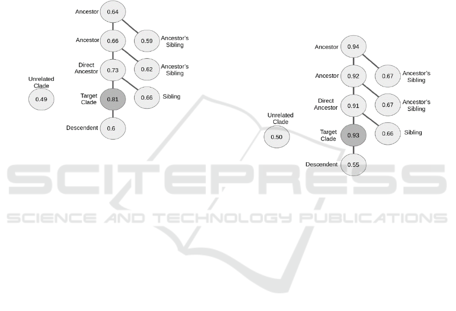
Figure 2: Tree representing the average MP-value for the
target clade (dark gray node) and taxonomic relatives. The
tree structure and labels of the nodes represents the
taxonomic relation. In this case, random sampling was
used.
Every dimension represents the membership
probability to a clade. That means only the random
forest classifiers that were trained on that particular
clade will influence this dimension. If the sample
originates from that clade, a high score is expected.
However, the scores of the dimensions that represent
a clade the sample does not belong to, are obtained by
classifiers that have never been trained using this
clade. This lead to random guessing (when leaving
taxonomic relatedness aside). Therefore, most
dimensions of the MP-vectors have random values.
This made clustering unsuccessful.
4.2 Random vs SMOTE Sampling
Even though the random sampling methods showed
good performances, with an hF measure of about 0.81
(Figure 2) there was a correlation between the hF
measure of the clades and their size (r = -0.7). That
indicated a classification problem as larger classes
had a worse hF score than smaller ones. This problem
probably resulted from under-sampling the larger
clade, so that not enough training samples for that
class were available. Also, one would expect that the
average MP-value of related species (especially
ancestors) would be higher than the obtained values.
This also indicates a methodological problem (Figure
2). When using SMOTE sampling, no such
correlation between clade size and hF measure could
be observed (data not shown), which indicates that
with this sampling method the class imbalance
problem has been overcome. Additionally, there
seems to be a taxonomic influence between predicted
and target species, because the average MP-values of
related species was higher than for unrelated species.
This would be expected especially for the ancestors,
as the target clade is always a member of the ancestor
clade (Figure 3).
Figure 3: Tree representing the average MP-value for the
target clade (dark gray node) and taxonomic relatives. The
tree structure and labels of the nodes represents the
taxonomic relation. In this case, SMOTE sampling was
used.
4.3 NewMIRBase Dataset
The performance on the newMiRBase dataset is
significantly poorer than on the MirBase dataset. This
difference in performance is partly due to many
sequences from unseen clades during training.
However, removing these sequences, the
performance still remains comparably poor. This is
likely caused by the origin of many of the sequences,
which are from species with few known members.
Therefore, the respective models have not seen
sufficient training data. These species are often only
present in clades of higher taxonomic layers.
Therefore, less RFs have been trained on the clade, so
that it is more difficult to obtain a reliable MP-value.
This also explains the discrepancy between the
AvgTPR rate and the hF measure in the newMiRBase
dataset.
A Machine Learning-based Approach for the Categorization of MicroRNAs to Their Species of Origin
155

4.4 Comparative Performance
Our approach performs better than BLAST on the
first mirBase dataset. -this holds for random and
SMOTE sampling. A comparison to other machine
learning approaches was not possible as this is the
first approach to address multi class species
categorization of miRNAs. However a comparison of
different two class classifiers (as a replacement for
the RFs) was performed only on homo sapiens
miRNAs (data not shown) with the best result being
obtained by the RF. This was confirmed by (Saçar &
Allmer, 2017), who trained different two class
classifiers on miRBase data for pre-miRNA
detection. However, in the future, it would be
interesting to train a common multi-class algorithm
like a SVM on the task for comparison. Interesting
would also be comparison with classifiers that where
designed for similar tasks (e.g. classification of
miRNA families).
5 CONCLUSIONS
MicroRNAs are regulators of gene expression and as
such important in cellular regulation and disease
(Tüfekci et al., 2014). Therefore, they are used for
investigating the molecular level of disease.
Experimental strategies must fail at detecting all
possible miRNA-mRNA interactions which is why
computational methods are used abundantly
(Demirci, Yousef & Allmer, 2019). Many
computational tools depend on data from online
resources such as miRBase. Unfortunately, databases
are not completely reliable, including miRNA
repositories. Some strategies associating miRNAs
with molecular events lead to questionable results
which is in part due to the smallness of miRNAs and
to the similarity among miRNAs exacerbated by
imperfect sequencing methods (Bağcı & Allmer,
2016). Additionally, miRNA evolution is not
completely unraveled and additional tools for its
investigation may be beneficial. We have succeed to
develop a machine learning approach that
successfully works on the microRNA species
categorization task. This approach tackles the three
issues outlined above. To the best of our knowledge
this is the only approach allowing for categorization
of miRNAs into their species of origin based only on
k-mer representation of the hairpin sequence. The
approach shall be used to assign a novel miRNA
sequence to the most closely clade to confirm that the
discovery is not a contamination. We also anticipate
that our approach could be used for the validation of
computational miRNA predictions by other tools.
Finally, the approach may be useful for further
investigation in miRNA evolution. However future
improvements need to address the introduction of
new or underrepresented species.
ACKNOWLEDGEMENTS
LO would like to thank Barbara Hammer,
Department of Machine Learning, University
Bielefeld for financial support. MY would like to
acknowledge Zefat Academic College for financial
support.
REFERENCES
Bağcı, C., & Allmer, J. (2016). One Step Forward, Two
Steps Back; Xeno-MicroRNAs Reported in Breast Milk
Are Artifacts. PLOS ONE, 11(1), e0145065.
https://doi.org/10.1371/journal.pone.0145065.
Bartel, D. P. (2009). MicroRNAs: target recognition and
regulatory functions. Cell, 136(2), 215–233.
https://doi.org/10.1016/j.cell.2009.01.002.
Berthold, M. R., Cebron, N., Dill, F., Gabriel, T. R., Kötter,
T., Meinl, T., … Wiswedel, B. (2008). KNIME: The
Konstanz Information Miner. In C. Preisach, H.
Burkhardt, L. Schmidt-Thime, & R. Decker (Eds.),
Data Analysis, Machine Learning and Applications
(pp. 319–326). Berlin, Heidelberg: Springer.
https://doi.org/10.1007/978-3-540-78246-9_38.
Chawla, N. V., Bowyer, K. W., Hall, L. O., & Kegelmeyer,
W. P. (2002). SMOTE: Synthetic Minority Over-
sampling Technique. Journal of Artificial Intelligence
Research, 16, 321–357. https://doi.org/10.1613/
jair.953.
Demirci, M. D. S., Yousef, M., & Allmer, J. (2019).
Computational Prediction of Functional MicroRNA–
mRNA Interactions. In Computational Biology of Non-
Coding RNA (pp. 175-196). Humana Press, New York,
NY.
Edgar, R. C. (2010). Search and clustering orders of
magnitude faster than BLAST. Bioinformatics, 26(19),
2460–2461. https://doi.org/10.1093/bioinformatics/
btq461
Fernández, A., López, V., Galar, M., del Jesus, M. J., &
Herrera, F. (2013). Analysing the classification of
imbalanced data-sets with multiple classes:
Binarization techniques and ad-hoc approaches.
Knowledge-Based Systems, 42, 97–110.
https://doi.org/10.1016/j.knosys.2013.01.018
Fiscon, G., Conte, F., Farina, L., Pellegrini, M., Russo, F.,
& Paci, P. (2019). Identification of Disease–miRNA
Networks Across Different Cancer Types Using
SWIM. In MicroRNA Target Identification (pp. 169-
181). Humana Press, New York, NY.
BIOINFORMATICS 2020 - 11th International Conference on Bioinformatics Models, Methods and Algorithms
156

Gordon, A. D. (1987). A review of hierarchical
classification. Journal of the Royal Statistical Society:
Series A (General), 150(2), 119-137.
Hammond, S. M. (2015). An overview of microRNAs.
Advanced Drug Delivery Reviews, 87, 3–14.
https://doi.org/10.1016/j.addr.2015.05.001
Hamzeiy, H., Suluyayla, R., Brinkrolf, C., Janowski, S. J.,
Hofestaedt, R., & Allmer, J. (2017). Visualization and
Analysis of MicroRNAs within KEGG Pathways using
VANESA. Journal of Integrative Bioinformatics,
14(1). https://doi.org/10.1515/jib-2016-0004
Kiritchenko, S., Matwin, S., Nock, R., & Famili, A. F.
(2006). Learning and Evaluation in the Presence of
Class Hierarchies: Application to Text Categorization.
In L. Lamontagne & M. Marchand (Eds.), Advances in
Artificial Intelligence (pp. 395–406). Springer Berlin /
Heidelberg.
Kozomara, A., & Griffiths-Jones, S. (2011). miRBase:
integrating microRNA annotation and deep-sequencing
data. Nucleic Acids Research, 39 (Database issue),
D152-7. https://doi.org/10.1093/nar/gkq1027
Kurtz, S., Narechania, A., Stein, J. C., & Ware, D. (2008).
A new method to compute K-mer frequencies and its
application to annotate large repetitive plant genomes.
BMC Genomics, 9(1), 517. https://doi.org/10.1186/
1471-2164-9-517
Meng, Y., Shao, C., Wang, H., & Chen, M. (2012). Are all
the miRBase-registered microRNAs true? A structure-
and expression-based re-examination in plants. RNA
Biology, 9(3), 249–253. https://doi.org/10.4161/
rna.19230
Rodriguez, A. (2004). Identification of Mammalian
microRNA Host Genes and Transcription Units.
Genome Research, 14(10a), 1902–1910. Retrieved
from http://www.ncbi.nlm.nih.gov/pubmed/15364901
Saçar Demirci, M. D., Baumbach, J., & Allmer, J. (2017).
On the performance of pre-microRNA detection
algorithms. Nature Communications, 8(1), 330.
https://doi.org/10.1038/s41467-017-00403-z
Saçar, M. D., & Allmer, J. (2014). Machine learning
methods for microRNA gene prediction. Methods in
Molecular Biology (Clifton, N.J.). https://doi.org/
10.1007/978-1-62703-748-8_10
Saçar, M. D., Hamzeiy, H., & Allmer, J. (2013). Can
MiRBase provide positive data for machine learning for
the detection of MiRNA hairpins? Journal of
Integrative Bioinformatics, 10(2), 215.
https://doi.org/10.2390/biecoll-jib-2013-215
Sempere, L. F., Cole, C. N., Mcpeek, M. A., & Peterson, K.
J. (2006). The phylogenetic distribution of metazoan
microRNAs: insights into evolutionary complexity and
constraint. Journal of Experimental Zoology Part B:
Molecular and Developmental Evolution, 306B
(6),
575–588. https://doi.org/10.1002/jez.b.21118
Takamizawa, J., Konishi, H., Yanagisawa, K., Tomida, S.,
Osada, H., Endoh, H., … Takahashi, T. (2004).
Reduced expression of the let-7 microRNAs in human
lung cancers in association with shortened
postoperative survival. Cancer Res, 64(11), 3753–
3756. https://doi.org/10.1158/0008-5472.CAN-04-
0637
Tanzer, A., & Stadler, P. F. (2004). Molecular evolution of
a microRNA cluster. Journal of Molecular Biology,
339(2), 327–335. https://doi.org/10.1016/j.jmb.2004.
03.065
Tin Kam Ho. (1995). Random decision forests. In
Proceedings of 3rd International Conference on
Document Analysis and Recognition (Vol. 1, pp. 278–
282). Montreal, Canada: IEEE Comput. Soc. Press.
https://doi.org/10.1109/ICDAR.1995.598994
Tüfekci, K. U., Oner, M. G., Meuwissen, R. L. J., & Genç,
S. (2014). The role of microRNAs in human diseases.
Methods in Molecular Biology (Clifton, N.J.), 1107,
33–50. https://doi.org/10.1007/978-1-62703-748-8_3
Xu, Q.-S., & Liang, Y.-Z. (2001). Monte Carlo cross
validation. Chemometrics and Intelligent Laboratory
Systems, 56(1), 1–11.
Yousef, M., Khalifa, W., Acar, E., & Allmer, J. (2017).
MicroRNA categorization using sequence motifs and k-
mers. BMC Bioinformatics, 18(1). https://doi.org/
10.1186/s12859-017-1584-1
Yousef, M., Nigatu, D., Levy, D., Allmer, J., & Henkel, W.
(2017). Categorization of species based on their
microRNAs employing sequence motifs, information-
theoretic sequence feature extraction, and k-mers.
Eurasip Journal on Advances in Signal Processing,
2017(1). https://doi.org/10.1186/s13634-017-0506-8
Yousef, Malik. (2019). Hamming Distance and K-mer
Features for Classification of Pre-cursor microRNAs
from Different Species. In C. Benavente-Peces, S. Ben
Slama, & B. Zafar (Eds.), Proceedings of the 1st
International Conference on Smart Innovation,
Ergonomics and Applied Human Factors (SEAHF) (pp.
180–189). Cham: Springer International Publishing.
Yousef, Malik, & Allmer, J. (2019). Classification of Pre-
cursor microRNAs from Different Species Using a New
Set of Features BT - Database and Expert Systems
Applications. In G. Anderst-Kotsis, A. M. Tjoa, & I.
Khalil (Eds.) (pp. 15–20). Cham: Springer International
Publishing.
Zhang, B., Pan, X., Cannon, C. H., Cobb, G. P., &
Anderson, T. A. (2006). Conservation and divergence
of plant microRNA genes. The Plant Journal, 46(2),
243–259.
A Machine Learning-based Approach for the Categorization of MicroRNAs to Their Species of Origin
157
