
CNN-based Deblurring of Terahertz Images
Marina Ljubenovi
´
c
a
, Shabab Bazrafkan
b
, Jan De Beenhouwer
c
and Jan Sijbers
d
imec-Vision Lab, Department of Physics, University of Antwerp, Belgium
{marina.ljubenovic, shabab.bazrafkan, jan.debeenhouwer, jan.sijbers}@uantwerpen.be
Keywords:
THz Imaging, THz-TDS, CNN, Deblurring.
Abstract:
The past decade has seen a rapid development of terahertz (THz) technology and imaging. One way of doing
THz imaging is measuring the transmittance of a THz beam through the object. Although THz imaging is a
useful tool in many applications, there are several effects of a THz beam not fully addressed in the literature
such as reflection and refraction losses and the effects of a THz beam shape. A THz beam has a non-zero
waist and therefore introduces blurring in transmittance projection images which is addressed in the current
work. We start by introducing THz time-domain images that represent 3D hyperspectral cubes and artefacts
present in these images. Furthermore, we formulate the beam shape effects removal as a deblurring problem
and propose a novel approach to tackle it by first denoising the hyperspectral cube, followed by a band by
band deblurring step using convolutional neural networks (CNN). To the best of our knowledge, this is the
first time that a CNN is used to reduce the THz beam shape effects. Experiments on simulated THz images
show superior results for the proposed method compared to conventional model-based deblurring methods.
1 INTRODUCTION
Terahertz (THz) technology, and especially THz
imaging has attracted increasing interest in recent
years, mostly due to immense progress in THz
sources development (Guillet et al., 2014). Many
imaging applications in security (Kemp et al., 2003),
conservation of cultural heritage (Cosentino, 2016),
and in many other fields, find their place within a
THz range (i.e., 0.1 to 10 THz). Additionally, such
increasing interest is attributed to the fact that a THz
beam is non-ionizing and can be applied to soft ma-
terials providing an alternative to X-ray in many ap-
plications (e.g., computed tomography (CT) (Recur
et al., 2012)). Moreover, THz technology is used
in spectroscopy for testing, imaging, analysing, and
chemical recognition of different materials (Baxter
and Guglietta, 2011).
While in recent years powerful THz detectors
have been developed and applied to imaging (El Fa-
timy et al., 2009), they are not yet fully integrated
with an array structure (Nadar et al., 2010; Burger
et al., 2019). Current detectors are usually one- to
few-pixels large, leading to a long scanning time
a
https://orcid.org/0000-0002-4404-3630
b
https://orcid.org/0000-0003-4561-7250
c
https://orcid.org/0000-0001-5253-1274
d
https://orcid.org/0000-0003-4225-2487
as for 2D images, an object needs to be scanned
pixel by pixel. Secondly, the propagation of a THz
beam through the object leads to the diffraction ef-
fect (Mukherjee et al., 2013) and Fresnel losses (Tepe
et al., 2017). Finally, the effects of a THz beam shape
additionally limit the achievable resolution. These ef-
fects cannot be neglected as the THz beam has a non-
zero waist (minimum beam radius) and therefore in-
troduces a blurring effect to the resulting image.
In recent years, several methods were proposed
to deal with the afore mentioned blurring effects and
to increase the spatial resolution of THz images. In
(Xu et al., 2014b), the authors employed several well-
known super-resolution approaches to THz images:
projection onto a convex set, iterative backprojec-
tion, Richardson–Lucy iterative approach (Richard-
son, 1972; Lucy, 1974), and 2D wavelet decompo-
sition reconstruction (Mallat, 2008). In (Popescu
and Hellicar, 2010), a method is presented for a
point-spread function (PSF) estimation by applying
a specially designed phantom. To validate PSF es-
timation, they perform several experiments apply-
ing a well-known Wiener deconvolution technique
(Dhawan et al., 1986). To deal with THz beam shape
effects in THz-CT, Recur et al. modelled a THz beam
and incorporated it in several well-established CT re-
construction approaches as a convolution filter (Recur
et al., 2012). Although these methods yield promis-
ing results, they are tailored to a single THz image
or a specific application (e.g., THz-CT). Furthermore,
conventional deconvolution approaches require one or
more input parameters that, in many cases, need to be
hand-tuned.
In this work, we propose a method for beam shape
effects removal from time-domain THz images that
represent a hyperspectral cube with several hundred
bands. The problem of beam shape effects removal
can be formulated as a deblurring task, also known as
deconvolution, with a known, band-dependant, PSF.
In fact, a cross-section of a THz beam at the object
position can be modelled as a Gaussian distribution
(Recur et al., 2012).
In the last few years, we are witnessing the rapid
development of deep learning and neural network-
based approaches for various computer vision tasks
(LeCun et al., 2015; Voulodimos et al., 2018). The
convolutional neural network (CNN) is arguably the
most common class of deep neural networks applied
to image restoration tasks, such as denoising (Zhang
et al., 2017) and deblurring (Xu et al., 2014a). Here,
we will show how a CNN-based deblurring approach
tailored to THz images can be applied to remove the
blurring effect of a Gaussian beam. By using CNN-
based deblurring, we avoid hand-tuning of the input
parameters as network weights can be learned from a
set of training images.
In Section 2, we start by introducing a
pulsed/time-domain THz system and show how the
time-domain THz images can be synthesized using
different artefacts (e.g., blur and noise). We also ex-
plain how the THz beam is typically modelled and pa-
rameterized and finally introduce a novel CNN-based
approach for removing its effects. Finally, we com-
pare results obtained by conventional approaches with
the proposed CNN-based method and demonstrate ro-
bustness to noise of the proposed approach. To the
best of our knowledge, this is the first time that a CNN
or any other deep learning approach is applied to de-
blur THz time-domain images.
2 THZ BEAM SHAPE EFFECTS
In this work, we consider only a pulsed/time-domain
THz system, and, therefore, we will briefly introduce
it in this section.
2.1 Time-domain THz Imaging
THz time-domain spectroscopy (THz-TDS) is a tech-
nique that can be used for spectroscopy and imaging
in the THz domain (Hu and Nuss, 1995). A typical
THz-TDS system employs an ultrashort pulsed laser
(with pulses duration of 1 ps or less) and an antenna
(e.g., low-temperature grown GaAs). The laser gen-
erates a series of pulses which is split into two halves:
one for THz generation and the second to gate a de-
tector. A THz detector receives the incoming radia-
tion only for very brief periods of time which leads to
sampling of the THz field at various delays. Finally,
the resulting pulse is transformed into the frequency
domain covering a broad range of frequencies (e.g.,
from 0.076 to 2 THz). For more information about
the THz-TDS system and beamforming we refer to
(Chan et al., 2007) and references therein.
The main advantage of THz-TDS is its ability to
measure both spectral amplitude and phase. The am-
plitude of a THz signal is correlated to the absorbtion
and the phase is correlated to the thickness and den-
sity of the scanned object. Another unique character-
istic of THz-TDS is the broad bandwidth of the THz
radiation which is valuable for spectroscopy as many
materials have a unique fingerprint in the THz domain
(Baxter and Guglietta, 2011). Furthermore, in order
to be suitable for imaging and to increase the spa-
tial resolution, an imaging system typically includes
focusing optics. Finally, an image is formed from
the full dataset which contains a complete THz time-
domain waveform, the amplitude and the phase, cor-
responding to each pixel of the image. Additionally,
we may choose to calculate transmittance and phase-
difference images by measuring a reference back-
ground by leaving the optical path open. The resulting
THz-TDS images is seen as a hyperspectral data cube
where every band represents an image on a different
frequency in a given range.
With the introduction of the focusing optics, the
focal spot of the THz beam at the place of the object
has a complicated characteristic which strongly de-
pends on its design and system frequencies. Images
formed from lower frequencies are more blurry as the
beam waist increases with decreasing frequency. The
high frequency bands on the other hand are less blurry
because of the smaller beam waist. However, these
high frequency bands are noisier as they have lower
amplitudes (Duvillaret et al., 2000). Figure 1 shows
three bands of a real amplitude THz-TDS image of a
leaf acquired in a transmittance mode (a THz beam is
transmitted through the object).
2.2 THz Beam Modelling
In THz-TDS imaging, the THz beam can be modelled
as a Gaussian distribution characterized by a beam
waist which is closely connected to a frequency of
the THz system (Recur et al., 2012). Following the
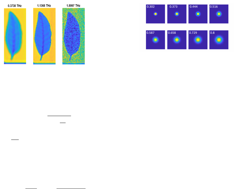
Figure 1: The THz-TDS amplitude image of a leaf at differ-
ent frequencies: left - 0.3738 THz (more blurry); middle -
1.1368 THz; right - 1.8997 THz (more noisy).
general beam modelling formulation, the radius at the
position x from the beam waist w
0
is
w(x) = w
0
r
1 + (
x
x
R
)
2
, (1)
where x
R
=
πw
2
0
λ
is the Rayleigh range with λ repre-
senting a wavelength. Furthermore, if I
0
represents
the beam intensity at the centre of w
0
and y and z are
distances from the beam axes in two directions, the
intensity distribution over cross-section in 3D is mod-
elled as
I(x,y,z) = I
0
w
0
w(x)
2
exp
−2(y
2
+ z
2
)
w
2
(x)
. (2)
We model the blurring artefacts present in one band
of THz-TDS images as the convolution between an
underlying sharp image and a known PSF
g = f ~ h + n, (3)
where g, f , h, and n represent one band of an observed
THz-TDS image, one band of an unknown sharp im-
age, a PSF (blurring operator), and noise respectively.
~ represents the convolution operator. Our goal is to
estimate the underlying sharp image f .
From (2) it is clear that several parameters define
the intensity within the beam: the wavelength (λ), the
beam waist (w
0
), and the intensity of the beam at w
0
(I
0
). We can set these parameters to control a PSF
model h which is used as a known variable in (3).
Note that the PSF represents an intersection of the 3D
THz beam in a position of the scanned object (see Fig-
ure 2).
The main goal of this work is to remove the blur-
ring effects from THz-TDS images. This is a chal-
lenging task as not only we have a different blur
(PSF) for different bands but also different noise lev-
els. Moreover, the size of each THz image band is
usually small (e.g., 61 × 41 pixels) which additionally
complicates a deblurring process. The differences in
blur and noise over bands and the small image size
Figure 2: Influence of a beam waist on PSF: Examples of
PSF for 1 THz, I
0
= 1, and different w
0
in mm (presented
with the numbers in the upper-left corner).
inspired us to propose a CNN-based deblurring ap-
proach: the proposed network is learned from a train-
ing dataset which contains all of these differences and
therefore it is arguably more robust than conventional
deblurring approaches.
3 CNN-BASED DEBLURRING
In the past few years, a new Machine Learning tech-
nique known as Deep Learning influenced a wide
range of experimental sciences with its revolution-
ary approach in solving signal processing problems
(Lemley et al., 2017). The main target of deep learn-
ing includes but is not limited to solving highly non-
linear, and sophisticated image processing problems
using a type of signal processing unit known as Deep
Neural Networks (DNN). These models consist of
different processing blocks such as fully connected,
convolution and deconvolution layers and pooling and
unpooling operations. DNNs provide superior results
in both classification and regression problems com-
pared to the classical machine learning approaches.
Applications such as object detection and classifica-
tion (Girshick, 2015; Ren et al., 2015; Redmon et al.,
2016), image segmentation for both medical (Ron-
neberger et al., 2015) and consumer (Varkarakis et al.,
2020; Badrinarayanan et al., 2017) use cases, and im-
age acquisition and reconstruction in CT (Bazrafkan
et al., 2019) are a few examples of Deep Learning im-
pacts on modern solutions for Image Processing ap-
plications.
In the current study, a fully convolutional DNN is
utilized to perform the deblurring operation to THz
images. A fully convolutional network only consists
of convolution and/or deconvolution layers with or
without pooling operations. All layers perform the
convolution operation with a learnable kernel which
is given by:
S
m
(x,y,c) = σ
n
m−1
c
∑
k=1
[n
w
/2]
∑
j=−[n
w
/2]
[n
h
/2]
∑
i=−[n
h
/2]
H
m
c
(i, j,k)·
S
m−1
(x − i,y − j,k)
,
(4)
where S
m
(i, j,c) is the signal in pixel location (x, y),
located in channel c in layer m, H
m
c
is the kernel
associated with the channel c of layer m. In other
words this kernel maps every channel in layer m − 1
to channel c in layer m. n
h
and n
w
are the width and
height of the kernel and n
m−1
c
is number of channels
in layer m − 1. σ is the activation function which is
also known as the nonlinearity of the layer.
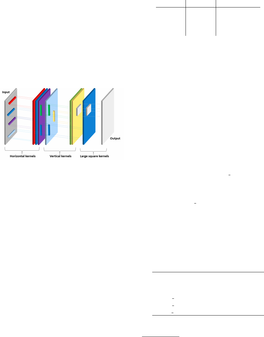
In (Xu et al., 2014a), the authors proposed a
network architecture designed for image deblurring.
This network is shown in Figure 3. The first two lay-
ers consist of horizontal and vertical kernels and the
last layer performs convolution with a large square
kernel. This design resembles the Singular Value De-
composition (SVD) technique used in conventional
deblurring methods, with the difference that here
these filters could be learned during training.
Figure 3: THzNet-2D architecture.
There are several other approaches for utilizing
DNNs to perform image deblurring (Tao et al., 2018;
Zhang et al., 2018). Nevertheless, we choose to use
the approach from (Xu et al., 2014a) as the pro-
posed network design is supported by the model-
based method (i.e., SVD) commonly used for image
restoration and therefore well studded.
4 EXPERIMENTS
To train and test a network, we created in total 8000
training and 200 test images corrupted by Gaussian
and Poisson noise and different blurs. We used these
two noise types to make the CNN more robust as
THz-TDS images in practice may be corrupted by
noise from several sources (Duvillaret et al., 2000).
Synthetic THz-TDS images (size: 61 × 41 × 263 pix-
els) are created by corrupting bands with different
blurs (controlled by different w
0
and λ as described
by Eq. (1)) and noise levels to simulate images as
described in Subsection 2.1. Frequencies over bands
(and therefore corresponding λ) are always set from
0.0076 to 1.9989 THz. The beam waists w
0
and in-
put noise levels over bands are randomly chosen from
sets presented in Table 1.
Table 1: Variations of w
0
, noise level for Gaussian noise,
and noise level for Poisson noise.
w
0
[mm] Gaussian Poisson (SNR)
1.5 - 0.5 0 68 - 13 dB
1.8 - 0.5 0 - 0.1 70 - 15 dB
1.5 - 0.3 0 - 0.2 72 - 17 dB
1.7 - 0.4 0 - 0.4 74 - 19 dB
The proposed approach contains two steps: in
the first step, we perform denoising as preprocess-
ing followed by the second step, CNN-based deblur-
ring. Denoising is performed using a state-of-the-art
hyperspectral image denoiser FastHyDe (Zhuang and
Bioucas-Dias, 2018) tailored to both Gaussian and
Poisson noise. Deblurring is performed band by band,
namely input and output of THzNet-2D is an image
corresponding to one band of a THz-TDS cube.
An ADAM optimizer (Kingma and Ba, 2014) was
utilized to update the network parameters with learn-
ing rate, β
1
, β
2
and ε equal to 0.00001, 0.9, 0.999, and
10
−8
, respectively. The MXNET 1.3.0 (Chen et al.,
2015)
1
framework was used to train the network on a
NVIDIA GTX 1070 in all the experiments.
To find optimal network settings we varied the
number and texture of training data and the approach
to weights initialization. These variations are listed in
Table 2. Note that in Table 2, 6k r stands for 6000
training images (6k THz-TDS cubes) from which 4k
is without texture and 2k is with background texture
that is extracted from real THz-TDS images. Simi-
larly, THzNet-2D-6k t contains 4k training data with-
out texture and 2k with synthetic texture (e.g., stripes,
dots). In every experiment, 20% of training images
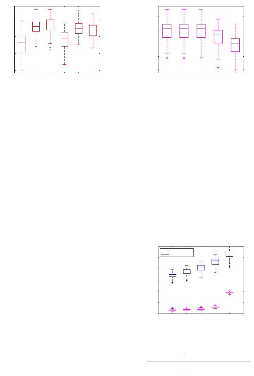
are used for validation. Comparison of the varia-
tions of THzNet-2D from Table 2 in terms of PSNR
is shown in Figure 4.
Table 2: THzNet-2D variations. NoI: Number of training
images; Init: Weights initialization method.
THzNet-2D NoI Texture Init
1k 1000 No Uniform
2k 2000 No Uniform
4k 4000 No Uniform
6k r 6000 Yes Uniform
6k t 6000 Yes Uniform
4k x 4000 No Xavier
Figure 4 shows the effect of the number and struc-
ture of a training data (note that the experiments are
1
https://mxnet.apache.org/
1k 2k 4k 6k_r 6k_t 4k_x
THzNet-2D Variations
16
18
20
22
24
26
28
30
PSNR
Figure 4: Comparison of different variations of THzNet-2D
(PSNR values obtained on the last band).
performed on the last band). Firstly, we can see how
the number of training data influnces the results (see
the results for THzNet-2D-4k compared to THzNet-
2D-2k). Secondly, the introduction of training data
with additional texture does not necessarily have a
positive influence on the results even if a test dataset
contains both images with and without texture. Fi-
nally, we tested the influence of a different initializa-
tion approach for network weights, a so-called Xavier
method (Glorot and Bengio, 2010) compared to the
uniform initialization.
Furthermore, we compared our THzNet-2D
network to conventional model-based deblur-
ring/deconvolution approaches: 1) Richardson-Lucy
method (RL) (Richardson, 1972; Lucy, 1974); 2)
RL followed by a state-of-the-art denoiser, BM3D
(Dabov et al., 2007) (RL+BM3D); 3) an extension
of BM3D for non-blind deblurring, IDD-BM3D
(Danielyan et al., 2012); 4) a state-of-the-art de-
blurring method with a hyper-Laplacian image prior
(H-L) (Krishnan and Fergus, 2009); and a well-
known Wiener deconvolution technique (Wiener)
(Dhawan et al., 1986).
The conventional methods were tested on 100
synthetic THz-TDS images. Deblurring of THz-
TDS images was performed band-by-band. Same as
previously, we applied a noise removal step using
FastHyDe method before deblurring. Furthermore,
we chose optimal parameters for all conventional de-
blurring approaches by measuring mean squared er-
ror (MSE) and peak signal-to-noise ratio (PSNR).
Results in terms of PSNR obtained with the model-
based deblurring approaches applied to the last band
(band 263) of 100 THz-TDS test images are presented
in Figure 5.
Figure 5 shows that RL, RL+BM3D, and IDD-
BM3D give the best results. These approaches are
not imposing a prior tailored to natural images: RL is
searching for a maximal likelihood solution without
the use of any prior knowledge and BM3D and IDD-
RL RL+BM3D IDD-BM3D H-L Wiener
Method
8
8.5
9
9.5
10
PSNR
Figure 5: Comparison of conventional model-based de-
blurring approaches (deblurring results obtained on the last
band).
BM3D are based on self-similarity of non-local im-
age patches. Here, we argue that this self-similarity
is present in THz images. On the contrary, the H-
L method imposes a hyper-Laplacian prior on im-
age gradients tailored to natural images. The Wiener
method expects an input parameter, noise-to-signal
power ratio, which is very difficult to tune for images
corrupted by moderate to strong noise.
Furthermore, in Figure 6 we show the difference
in performance of the RL method and THzNet-2D-
4k for different bands (namely bands 50, 100, 150,
200, and 263) and 100 THz-TDS images. We choose
RL and THzNet-2D-4k as they are arguably the best
tested model-based and CNN-based methods respec-
tively. Moreover, the average difference in perfor-
mance for the last band of the same 100 images mea-
sured by three metrics, MSE, PSNR, and structural
similarity index (SSIM) is shown in Table 3.
50 100 150 200 263
Bands
0
5
10
15
20
25
30
PSNR
THzNet-2D
Richardson-Lucy
Figure 6: THzNet-2D vs Richardson-Lucy in terms of
PSNR for different bands (50, 100, 150, 200, and 263).
Table 3: THzNet-2D vs Richardson-Lucy.
Method MSE PSNR SSIM
RL 0.113 9.475 0.544
THzNet-2D 0.002 26.673 0.929
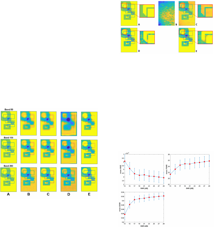
Figure 6 and Table 3 show that THzNet-2D out-
performs significantly the model-based method for
several tested bands. We also see that for higher bands
there is a better performance which is expected as they
are less blurry and the noise is mostly removed during
preprocessing.
Figure 7 illustrates the performance of THzNet-
2D for bands 50, 150, and 263. The first column
shows the ground truth bands and the second col-
umn represents the same bands with added blur and
noise. Furthermore, in the third column, we show the
results after preprocessing/denoising and finally, the
fourth and fifth columns show results obtained by the
RL method and THzNet-2D, respectively. The results
obtained by the RL method indicates strong ringing
and boundary artefacts. Boundary artefacts are most
likely due to the incorrect assumption of cyclic convo-
lution in (3). THzNet-2D output bands do not suffer
from the same artefacts. Nevertheless, we see that for
the lower band (band 50), the network output shows
some missing pixels especially visible on squared ob-
jects. Note that these square objects are only one pixel
thick.
Figure 7: THzNet-2D visual results for bands 50, 150, and
263 (first, second, and third rows respectively): A: Ground
truth; B: Blurry and noisy THz-TDS image; C: Blurry de-
noised THz-TDS image (THzNet-2D input); D: RL estima-
tion; E: THzNet-2D output.
To show the influence of texture on deblurring
results, we tested THzNet-2D on an image without
any texture and with added texture pattern. Figure 8
shows the texture pattern and the obtained results. In
the first row, we see the original ground truth image
without texture (A), followed by the texture pattern
(B), and the ground truth image with the added pat-
tern (C). Note that the contrast in the image C is in-
creased for the illustration purpose. The second row
represents the THzNet-2D output obtained on the last
band of the two THz-TDS images synthesized from
the above ground truths (D and E). The network out-
puts are comparable with the small differences visible
near the object edges.
Figure 8: Influence of texture on deblurring results. A:
Ground truth without texture; B: added texture pattern; C:
Ground truth with texture; D: THzNet-2D output tested on
image A (band 263); E: THzNet-2D output tested on image
C (band 263).
Finally, to test robustness to noise, we tested
THzNet-2D on images corrupted originally by Pois-
son noise with different noise levels (i.e., SNR of the
last band is from 29 to 13 dB). Although, the noise is
mostly removed during preprocessing it is interesting
to see its influence on the network performance. Fig-
ure 9 shows that the network performance decreases
only for very high noise levels (e.g., SNR = 15 and 13
dB). To emphasize this result, in Figure 10, we illus-
trate THzNet-2D output of the last band for different
input noise levels.
Figure 9: Robustness to noise: Mean MSE, PSNR, and
SSIM for the last band of 100 test images. The x axis is
the Poisson noise SNR in dB.
5 CONCLUSION
In this work, we propose a novel CNN-based ap-
proach for deblurring THz-TDS images. We showed
the superiority of the proposed method tested on syn-
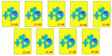
Figure 10: Robustness to noise: THzNet-2D output visual
results. Input noise levels in dB presented with numbers in
the bottom-right corner.
thetic images and compared to conventional model-
based deblurring methods in performing 2D-based
deblurring. There are several reasons for choosing
CNN-based approach, to name only two: i) CNNs are
robust to small-size and low-resolution images and ii)
there is no need for parameter settings as the network
weights are learned from training data. A drawback
of the proposed THzNet-2D network is reflected in
the process of creating realistic and sufficient train-
ing data. That is, training images need to resemble
real THz-TDS images as close as possible in terms
of size, artefacts (e.g., blur and noise), texture, and
intensity levels. Therefore, our current work covers
creating more complex intensity patterns and more
realistic training data. This is an important task as it
will provide a step towards testing the proposed CNN-
based approach on real data. Nevertheless, the pro-
posed CNN-based deblurring method can be seen as
a proof of concept: we show that employing a neural
network-based approach improve deblurring results
significantly.
Finally, there are at least two possible extensions
of THzNet-2D. The first one, covered by our current
work, is an extension of the network to perform de-
blurring on all bands jointly. By doing this, the net-
work may be able to learn connections between bands
during training. The second extension will include de-
noising into a deblurring process: instead of perform-
ing denoising as preprocessing, the network should
learn to perform both tasks denoising and deblurring.
ACKNOWLEDGEMENTS
The research leading to these results was part of the
IMEC-B-budget Tera-Tomo project (project number
41672). We thank Pavel Paramonov from Visan Lab
for fruitful discussions. We also thank Bert Gy-
selinckx and Lei Zhang from imec USA and Sachin
Kasture, Roelof Jansen, and Xavier Rottenberg from
imec for discussions and help with data acquisition.
REFERENCES
Badrinarayanan, V., Kendall, A., and Cipolla, R. (2017).
Segnet: A Deep Convolutional Encoder-Decoder Ar-
chitecture for Image Segmentation. IEEE Transac-
tions on Pattern Analysis and Machine Intelligence,
39(12):2481–2495.
Baxter, J. B. and Guglietta, G. W. (2011). Terahertz Spec-
troscopy. Analytical Chemistry, 83(12):4342–4368.
Bazrafkan, S., Van Nieuwenhove, V., Soons, J., De Been-
houwer, J., and Sijbers, J. (2019). Deep Neural Net-
work Assisted Iterative Reconstruction Method for
Low Dose CT. arXiv preprint arXiv:1906.00650.
Burger, M., F
¨
ocke, J., Nickel, L., Jung, P., and Augustin, S.
(2019). Reconstruction Methods in THz Single-Pixel
Imaging, pages 263–290. Springer International Pub-
lishing, Cham.
Chan, W. L., Deibel, J., and Mittleman, D. M. (2007). Imag-
ing with Terahertz Radiation. Reports on Progress in
Physics, 70(8):1325–1379.
Chen, T., Li, M., Li, Y., Lin, M., Wang, N., Wang, M., Xiao,
T., Xu, B., Zhang, C., and Zhang, Z. (2015). Mxnet: A
Flexible and Efficient Machine Learning Library for
Heterogeneous Distributed Systems. arXiv preprint
arXiv:1512.01274.
Cosentino, A. (2016). Terahertz and Cultural Heritage Sci-
ence Examination of Art and Archaeology. Technolo-
gies, 4(1):1–13.
Dabov, K., Foi, A., Katkovnik, V., and Egiazarian, K.
(2007). Image Denoising by Sparse 3-D Transform-
Domain Collaborative Filtering. IEEE Transactions
on Image Processing, 16(8):2080–2095.
Danielyan, A., Katkovnik, V., and Egiazarian, K. (2012).
BM3D Frames and Variational Image Deblurring.
IEEE Transactions on Image Processing, 21(4):1715–
1728.
Dhawan, A., Rangayyan, R., and Gordon, R. (1986). Im-
age Restoration by Wiener Deconvolution in Limited-
View Computed Tomography. Applied optics,
24(23):4013.
Duvillaret, L., Garet, F., and Coutaz, J.-L. (2000). Influ-
ence of Noise on the Characterization of Materials by
Terahertz Time-Domain Spectroscopy. Journal of the
Optical Society of America B, 17(3):452–461.
El Fatimy, A., Delagnes, J.-C., Younus, A., Nguema, E.,
Teppe, F., Knap, W., Abraham, E., and Mounaix, P.
(2009). Plasma Wave Field Effect Transistor as a Res-
onant Detector for 1 Terahertz Imaging Applications.
Optics Communications, 282(15):3055–3058.
Girshick, R. (2015). Fast R-CNN. In Proceedings of the
IEEE International Conference on Computer Vision,
pages 1440–1448.
Glorot, X. and Bengio, Y. (2010). Understanding the Diffi-
culty of Training Deep Feedforward Neural Networks.
In AISTATS, volume 9 of JMLR Proceedings, pages
249–256.
Guillet, J. P., Recur, B., Frederique, L., Bousquet, B.,
Canioni, L., Manek-H
¨
onninger, I., Desbarats, P., and
Mounaix, P. (2014). Review of Terahertz Tomogra-
phy Techniques. Journal of Infrared, Millimeter and
Terahertz Waves, 35(4):382–411.
Hu, B. B. and Nuss, M. C. (1995). Imaging with Terahertz
Waves. Optics Letters, 20(16):1716–1718.
Kemp, M. C., Taday, P. F., Cole, B. E., Cluff, J. A., Fitzger-
ald, A. J., and Tribe, W. R. (2003). Security Applica-
tions of Terahertz Technology. In Terahertz for Mil-
itary and Security Applications, volume 5070, pages
44–52.
Kingma, D. P. and Ba, J. (2014). Adam: A
Method for Stochastic Optimization. arXiv preprint
arXiv:1412.6980.
Krishnan, D. and Fergus, R. (2009). Fast Image Deconvo-
lution using Hyper-Laplacian Priors. In Advances in
Neural Information Processing Systems, pages 1033–
1041.
LeCun, Y., Bengio, Y., and Hinton, G. E. (2015). Deep
Learning. Nature, 521(7553):436–444.
Lemley, J., Bazrafkan, S., and Corcoran, P. (2017). Deep
Learning for Consumer Devices and Services: Push-
ing the limits for machine learning, artificial intelli-
gence, and computer vision. IEEE Consumer Elec-
tronics Magazine, 6(2):48–56.
Lucy, L. B. (1974). An Iterative Technique for the Recti-
fication of Observed Distributions. The Astronomical
Journal, 79(6):745–754.
Mallat, S. (2008). A Wavelet Tour of Signal Processing,
Third Edition: The Sparse Way. Academic Press, Inc.,
Orlando, FL, USA, 3rd edition.
Mukherjee, S., Federici, J., Lopes, P., and Cabral, M.
(2013). Elimination of Fresnel Reflection Boundary
Effects and Beam Steering in Pulsed Terahertz Com-
puted Tomography. Journal of Infrared, Millimeter,
and Terahertz Waves, 34(9):539–555.
Nadar, S., Videlier, H., Coquillat, D., Teppe, F., Sakow-
icz, M., Dyakonova, N., Knap, W., Seliuta, D., and
Ka
ˇ
salynas, I. (2010). Room Temperature Imaging at
1.63 and 2.54 THz with Field Effect Transistor Detec-
tors. Journal of Applied Physics, 108(5):054508.
Popescu, D. C. and Hellicar, A. D. (2010). Point Spread
Function Estimation for a Terahertz Imaging System.
EURASIP Journal on Advances in Signal Processing,
2010(1):575817.
Recur, B., Guillet, J. P., Manek-H
¨
onninger, I., Delagnes,
J. C., Benharbone, W., Desbarats, P., Domenger, J. P.,
Canioni, L., and Mounaix, P. (2012). Propagation
Beam Consideration for 3D THz Computed Tomog-
raphy. Optics Express, 20(6):5817–5829.
Redmon, J., Divvala, S., Girshick, R., and Farhadi, A.
(2016). You Only Look Once: Unified, Real-Time
Object Detection. In Proceedings of the IEEE Con-
ference on Computer Vision and PatternRecognition,
pages 779–788.
Ren, S., He, K., Girshick, R., and Sun, J. (2015). Faster R-
CNN: Towards Real-Time Object Detection with Re-
gion Proposal Networks. In Advances in Neural Infor-
mation Processing Systems, pages 91–99.
Richardson, W. H. (1972). Bayesian-Based Iterative
Method of Image Restoration. Journal of the Optical
Society of America, 62(1):55–59.
Ronneberger, O., Fischer, P., and Brox, T. (2015). U-Net:
Convolutional Networks for Biomedical Image Seg-
mentation. In International Conference on Medical
Image Computing and Computer-Assisted Interven-
tion, pages 234–241.
Tao, X., Gao, H., Shen, X., Wang, J., and Jia, J. (2018).
Scale-Recurrent Network for Deep Image Deblurring.
In Conference on Computer Vision and Pattern Recog-
nition, pages 8174–8182.
Tepe, J., Schuster, T., and Littau, B. (2017). A Modified Al-
gebraic Reconstruction Technique Taking Refraction
Into Account with an Application in Terahertz Tomog-
raphy. Inverse Problems in Science and Engineering,
25(10):1448–1473.
Varkarakis, V., Bazrafkan, S., and Corcoran, P. (2020).
Deep Neural Network and Data Augmentation
Methodology for Off-Axis Iris Segmentation in Wear-
able Headsets. Neural Networks, 121:101–121.
Voulodimos, A., Doulamis, N., Doulamis, A., and Protopa-
padakis, E. (2018). Deep Learning for Computer Vi-
sion: A Brief Review. Computational Intelligence and
Neuroscience, 2018:1–13.
Xu, L., Ren, J. S. J., Liu, C., and Jia, J. (2014a). Deep
Convolutional Neural Network for Image Deconvolu-
tion. In Advances in Neural Information Processing
Systems 27, pages 1790–1798. Curran Associates, Inc.
Xu, L.-M., Fan, W., and Liu, J. (2014b). High-Resolution
Reconstruction for Terahertz Imaging. Applied Op-
tics, 53(33):7891–7897.
Zhang, J., Pan, J., Ren, J., Song, Y., Bao, L., Lau, R. W. H.,
and Yang, M. (2018). Dynamic Scene Deblurring Us-
ing Spatially Variant Recurrent Neural Networks. In
2018 IEEE/CVF Conference on Computer Vision and
Pattern Recognition, pages 2521–2529.
Zhang, K., Zuo, W., Chen, Y., Meng, D., and Zhang, L.
(2017). Beyond a Gaussian Denoiser: Residual Learn-
ing of Deep CNN for Image Denoising. IEEE Trans-
actions on Image Processing, 26(7):3142–3155.
Zhuang, L. and Bioucas-Dias, J. M. (2018). Fast Hyper-
spectral Image Denoising and Inpainting Based on
Low-Rank and Sparse Representations. IEEE Jour-
nal of Selected Topics in Applied Earth Observations
and Remote Sensing, 11(3):730–742.
