Detecting and Locating Boats using a PTZ Camera with Both Optical
and Thermal Sensors
Christoffer P. Simonsen
a
, Frederik M. Thiesson
b
, Øyvind Holtskog
c
and Rikke Gade
d
Department of Architecture, Design and Media Technology, Aalborg University, Fredrik Bajers Vej, Aalborg, Denmark
Keywords:
Object Detection, CNN, PTZ Camera, Transfer-learning, Thermal Camera, Single Camera Positioning,
Ray-casting.
Abstract:
A harbor traffic monitoring system is necessary for most ports, yet current systems are often not able to detect
and receive information from boats without transponders. In this paper we propose a computer vision based
monitoring system utilizing the multi-modal properties of a PTZ (pan, tilt, zoom) camera with both an optical
and thermal sensor in order to detect boats in different lighting and weather conditions. In both domains boats
are detected using a YOLOv3 network pretrained on the COCO dataset and retrained using transfer-learning
to images of boats in the test environment. The boats are then positioned on the water using ray-casting. The
system is able to detect boats with an average precision of 95.53% and 96.82% in the optical and thermal
domains, respectively. Furthermore, it is also able to detect boats in low optical lighting conditions, without
being trained with data from such conditions, with an average precision of 15.05% and 46.05% in the optical
and thermal domains, respectively. The position estimator, based on a single camera, is able to determine the
position of the boats with a mean error of 18.58 meters and a standard deviation of 17.97 meters.
1 INTRODUCTION
Port traffic management is a crucial operation in large
ports and is given much attention throughout the
world (Branch, 1986). The aim of such a system is to
use all sources of information in order to build a com-
prehensive situation awareness (Council of the Euro-
pean Union, 2008). Current major ports use moni-
toring systems for large industrial or passenger boats.
Well-trained human operators use sophisticated tools
at their disposal in order monitor all activity within
their area. These tools include: radars, information
systems, and a large number of communication tools,
which are all aiding the operators in providing infor-
mation on request and coordinate movement of boats
(Wiersma and Mastenbroek, 1998). However, smaller
ports experience traffic from a large variety of ves-
sels, ranging from cargo/cruise ships to small kayaks.
The smaller vessels are not necessarily equipped with
transponders and are therefore most often overlooked
in these monitoring systems. Computer vision based
a
https://orcid.org/0000-0002-1192-9670
b
https://orcid.org/0000-0001-8235-036X
c
https://orcid.org/0000-0001-8092-6468
d
https://orcid.org/0000-0002-8016-2426
solutions have the potential to overcome the problem
of locating vessels with no transponders. With the use
of cameras, it is possible to detect and determine the
position of boats of almost any size in a port with-
out the use of transponders. However, it is important
that the system works in all weather and lighting con-
ditions. Sole use of an optical sensor would likely
fail to detect boats in poor lighting conditions, such
as during the night or in heavy rain. This leads us to
our proposed computer vision based solution.
In this paper we propose a marine monitoring sys-
tem that, with the use of a bi-spectrum camera, can
detect and estimate the position of boats in different
weather and light conditions. We begin our paper by
presenting existing vision based monitoring solutions
and address their problems in Section 2. This is fol-
lowed by an explanation of our hardware setup and
image calibration in Section 3. The boat detection
method is described in Section 4 and the position es-
timation of detected boats is presented in Section 5.
Finally, the conclusion and discussion is found in Sec-
tion 6. The flow of the system is to first acquire im-
ages from each sensor, correct them for distortion, and
register them. Boats are then detected in each image
separately and subsequently fused in order to not de-
termine the position of the same boat twice. Lastly

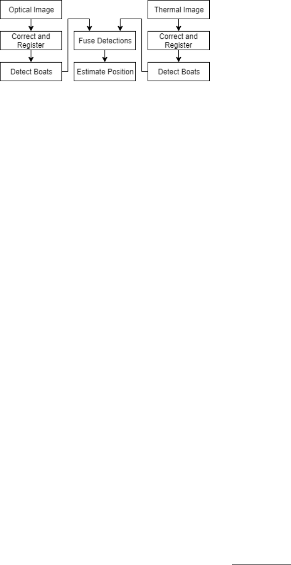
the boats position is estimated utilizing the predicted
bounding box positions. The flow of the system is
illustrated in the diagram in Figure 1.
Figure 1: The system flow.
The contributions of this paper are as follows:
• We present a boat detection method robust to
changing lighting conditions.
• We show that a pretrained Convolutional Neural
Network (CNN) based detector can be fine-tuned
to the thermal domain using limited training data.
• We propose and evaluate a ray-casting method for
positioning boats with a PTZ camera.
2 RELATED WORK
Overview of Detection Methods. Within the past
20 years, object detection has progressed from
traditional detection methods such as Viola Jones
Detectors (Viola and Jones, 2001) and HOG De-
tectors (Dalal and Triggs, 2005), to deep learning
detection methods (Zou et al., 2019), predominantly
based on the use of convolutional neural networks
(CNNs) (Chen et al., 2019)(Zhu et al., 2018). With
the large amounts of annotated data available, as
well as accessible GPUs with high computational
capabilities, a deep learning era began where object
detection started to evolve at an unprecedented speed
(Zou et al., 2019) (Liu et al., 2018). However, there
is no universal solution able to solve all detection
tasks. This is due to a speed/accuracy trade-off where
CNNs that perform faster tend to be less accurate than
their more complex and computationally expensive
counterparts (Huang et al., 2017). Two-stage region
proposal object detectors such as R-CNNs (Girshick
et al., 2013), tend to have great accuracy but require
thousands of network evaluations for a single image
proving to be computationally expensive (Redmon
et al., 2016)(Redmon and Farhadi, 2017). In contrast,
one-stage object detectors such as Single Shot
MultiBox Detector (Liu et al., 2016), provide faster
detection which comes at the price of accuracy
(Huang et al., 2017). Akiyama et al. proposed a boat
detector based on a custom CNN model trained on
RGB images from a surveillance camera (Akiyama
et al., 2018). Their model scored an average F1-score
of 0.70, but they did not test on any images captured
in poor lighting conditions.
Overview of Localization Methods. Global
Positioning System (GPS) localization systems are
popular in a plethora of applications (Drawil et al.,
2013). But as previously mentioned smaller vessels
are often not equipped with GPS and transponders.
Presented with two cameras viewing the same
reference point, stereo vision is one method for
estimating the position of objects for computer vision
applications. This is done by matching images
from different viewpoints (Mohan and Ram, 2015).
However, if the cameras operate in different spectra,
then depth map based texture matching is difficult
to construct, especially with the complexity of the
scene. Homography is another method which could
be used for localization. The main advantage is a
single camera can be used to estimate the position
to objects. In this method, the image coordinates
are mapped to the coordinates of a known plane
(Agarwal et al., 2005). Yet the problem with this
method is that the camera must be fixed in a single
position (Agarwal et al., 2005), which would limit
the pan and tilt functionality of the PTZ camera. One
method often used in video games to determine if
and how to render objects, based on the camera’s
distance and orientation in respect to the object, is
ray-casting. This method is applicable using a single
camera and allows for camera movement. It requires
objects to be defined in 3D space to determine the
rays intersection with them and hence evaluate their
position in relation to the camera (Hughes et al.,
2013).
3 SETUP AND CALIBRATION
The camera used is a Hikvision DS-2TD4166-50
1
.
The camera is bi-spectrum with an optical and ther-
mal sensor. The thermal sensor is beneficial as it
is independent on external optical light sources and
instead utilizes the infrared radiation from objects
within the field of view (Gade and Moeslund, 2014).
The Hikvision camera is mounted on a dome, which
allows for manipulation of the camera orientation
with two degrees of freedom: pan (left/right move-
ment) and tilt (up/down movement). The dome is
mounted on top of a building with an overview of
a small port, which is visited by everything from
cruise ships to kayaks. The camera is connected to a
1
Specification list found at (Hikvision, 2019)

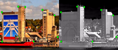
(a) Optical image. (b) Thermal image.
Figure 2: An example of potential feature points indicated
by the green circles.
computer with the following specifications: Intel(R)
Xeon(R) CPU E5-1620 v4 @ 3.50 GHz, 16.0 GB
RAM, Nvidia GeForce GTX 1080 Ti GPU and op-
erating on Windows 10 (64-bit). Both the optical and
thermal sensor information will be used in order to
create a system which is more robust to environmen-
tal conditions. Therefore, the output of the system
will be based on a late-fusion of the information of the
two sensors. To allow fusion of the sensor informa-
tion, the images must be registered to the same image
plane. Firstly, the intrinsic parameters of the two sen-
sors are calibrated separately. Secondly, the images
are aligned by performing image registration. The
calibration of the cameras was done using a checker-
board and Zhang’s method (Zhang, 2000). Detecting
the checkerboard using an optical sensor is straight-
forward, however, since the thermal sensor captures
temperature differences instead of colours, in many
conditions a regular checkerboard may seem uniform
to the thermal camera. Yet since the calibration was
done outside the light from the sun would heat the
black tiles more than the white tiles and an inverse
version of the checkerboard was visible. The issue
of calibrating thermal cameras and different solutions
are discussed in (Gade and Moeslund, 2014). The so-
lution for our system is similar to the one presented
in (John et al., 2016). After correcting the images for
potential distortion, they can be registered. The opti-
cal image will be registered onto the thermal image.
This is done since the thermal sensor has a fixed focal
length with a known value which will be desirable for
later boat position estimation. The images were reg-
istered by performing an affine transformation on the
optical image. In order to determine the transforma-
tion, a feature based approach was used (Goshtasby,
1988)(Goshtasby, 1986). In this approach several cor-
responding feature points are selected manually from
both images. The feature points chosen were points
such as roof tops and chimneys since these where
clearly visible in both images and the points were cho-
sen to span as much of the images as possible. Figure
2 shows feature points in the two images.
4 DETECTOR
For this work, we need the system to perform boat
detection in two individual video streams at real time.
Furthermore, as small ports and the surrounding wa-
ters may experience fast moving boats, like motor-
boats, the system should run at a high enough frame
rate to provide smooth localizations of all boats. This
suggests the use of a one stage CNN detector. The one
stage object detector chosen was YOLO (You Only
Look Once)(Redmon and Farhadi, 2018). The details
will be described in the following section.
4.1 Implementation
There are various implementations of YOLO, each
with varying architectures and trained on different
datasets for unique applications. Recently, YOLO
version 3 (YOLOv3) was released which improved
not only the speed but also the accuracy of the previ-
ous YOLOv2 (Redmon and Farhadi, 2018). Further-
more, when processing 320 × 320 images, YOLOv3
runs as accurate as Single Shot MultiBox Detector
(Liu et al., 2016), but three times faster (Redmon
and Farhadi, 2018). For the purposes of our system,
the YOLOv3 subvariant chosen was the pre-trained
YOLOv3-416 model with 416 × 416 input image size
with weights pre-trained on the Common Objects in
Context (COCO) Dataset (Lin et al., 2014). The in-
put image size was chosen to be as great as possi-
ble while still maintaining a high frame rate applica-
tion. The COCO dataset was chosen as it already has
a ’boat’ class. Henceforth, when YOLOv3 is men-
tioned throughout this paper, it refers to the YOLOv3-
416 model. With the pre-trained YOLOv3 model, a
preliminary performance evaluation on both optical
and thermal images of boats was done.
4.1.1 Preliminary Evaluation
To evaluate the performance of the pre-trained
YOLOv3 model, the COCO metrics will be calcu-
lated. Specifically Average Precision (AP) which
is calculated by combining the metrics ”precision”,
”recall” and ”Intersection over Union” into a single
quantity as shown in (Zhang and Zhang, 2009), where
the greater the metric, the better the model. AP is
calculated for a single class whereas mean Average
Precision (mAP) is calculated by taking the mean of
all APs from all classes. In order to evaluate pre-
trained YOLOv3’s performance on our setup we col-
lected data from our setup manually saving both the
optical and thermal image whenever a boat was seen.
This resulted in two separate datasets, one for optical
images and one for the thermal counterpart, where a

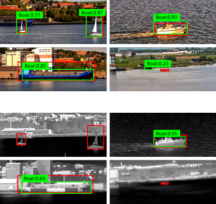
small subset of each can be seen in Figure 3. The red
boxes in Figure 3 indicate the ground truth bound-
ing box positions of the boats. 288 images for each
modality were collected. Following the evaluation
metrics set by COCO, the AP was calculated with an
IoU threshold of 50% and precision and recall were
calculated with a confidence threshold of 25%. Us-
ing the testing dataset for optical images resulted in
an AP score of 75.58% for boats. An example of run-
ning YOLOv3 on the optical images can be seen in
Figure 3a, indicated by the green boxes. Using the
testing dataset for thermal images resulted in an AP
score of 36.42% for boats. This lesser result, com-
pared to the optical data, is to be expected as YOLOv3
is trained using the COCO dataset which is composed
solely of optical images and not thermal images. An
example of running YOLOv3 on the thermal images
can be seen in Figure 3b. To better adapt the detector
to the thermal domain, YOLOv3 should be retrained
with a set of thermal images. Furthermore, although
pre-trained YOLOv3 on optical images had and AP
score of 75.58%, it will also be retrained in order to
further improve it.
(a) Optical images as input.
(b) Thermal image as input.
Figure 3: Output of the YOLOv3 model pretrained on the
COCO dataset. The red boxes are the ground truth annota-
tions, while the green boxes are the detections.
4.2 Retraining YOLO
In order to retrain a YOLOv3 model for each modal-
ity, more data was collected. This resulted in 640
pairs of images, in addition to the preliminary test
dataset of 288 images. With these small datasets,
transfer learning is utilized in order to avoid retrain-
ing the entire model, which requires large amounts of
data. When performing transfer learning, certain lay-
ers of the model are frozen, where a frozen layer does
not change weights during the training process. The
rule of thumb is that the more data available, the less
layers should be frozen (Yosinski et al., 2014). As
our datasets are limited, it is suggested to freeze the
entire feature extractor of the object detector in order
to avoid overfitting when training the models (Yosin-
ski et al., 2014). This is also known as fine-tuning the
model. This is the approach taken for the purposes of
retraining YOLOv3. We retrain the YOLOv3 network
to detect only a single class: ”boat”.
4.2.1 Training
We trained YOLOv3 with an approximately 70/30
(450 and 190 images) split between training data and
validation data. The split was done to ensure that the
validation dataset contained boats not present in the
training dataset. To determine when to stop training
each model, the evaluation metrics AP and loss error
were used. The loss error is the output from the cost
function of the model where the lower the error, the
better the model. Hence, training should be stopped
at the greatest AP and lowest loss error. A maximum
AP of 98% and 97% were reached for the optical and
thermal models, respectively, where no further signif-
icant decrease in loss was observed.
4.2.2 Evaluation
In order to evaluate the two retrained YOLOv3 mod-
els for optical and thermal images, the same evalua-
tion metrics and dataset from the preliminary evalu-
ation in Section 4.1.1 was used. The fine-tuned op-
tical YOLOv3 model had an AP of 95.53% whereas
the YOLOv3 model pretrained on the COCO dataset
scored an AP of 75.58%. The fine-tuned thermal
YOLOv3 model scored an AP of 96.82%, which is a
significant increase compared to the model pretrained
on the COCO dataset, which scored an AP of 36.42%
on the thermal data. The AP scores were calculated
with an IoU threshold of 50%. The average IoU was
also measured as it gives an indication of how pre-
cise the position of the boats can be estimated. The
average IoU was 72.36% and 74.14% for the opti-
cal and thermal model, respectively. Figure 4 and 5
show some qualitative results on optical and thermal
images, respectively.
4.3 Poor Optical Lighting Test
A test was conducted to compare the performance of
the models in poor lighting conditions. A dataset was

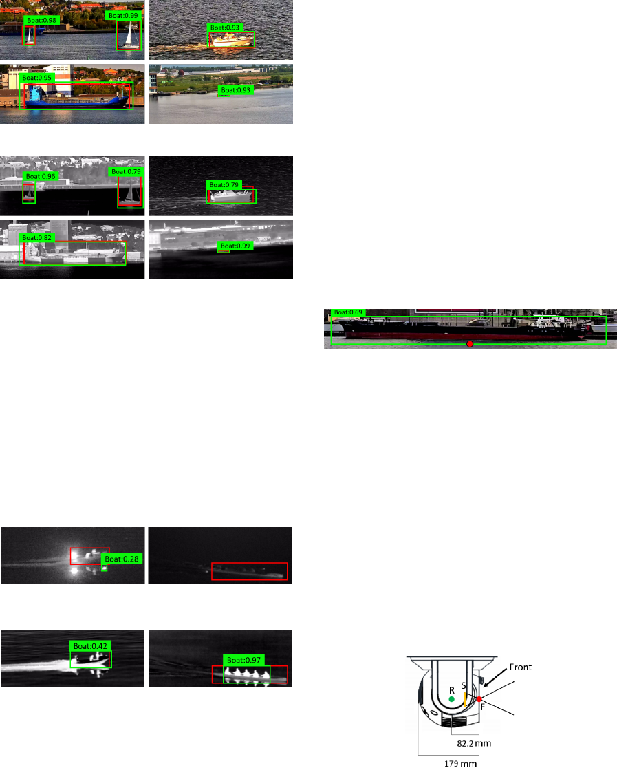
Figure 4: Output of retrained YOLOv3 on optical images.
Figure 5: Output of retrained YOLOv3 on thermal images.
collected containing 24 pairs of images of boats dur-
ing the night. This dataset is rather small since only
a few boats were present during the night. The night
dataset was processed by the two fine-tuned models
scoring an AP of 15.05% and 46.05% for the opti-
cal and thermal model, respectively. Both scores are
lower than the evaluation with images captured during
daytime but it is clear that the thermal model is out-
performing the optical model under low optical light
conditions. Examples of processed night images are
presented in Figure 6 and Figure 7, where the red
boxes indicate the ground truth and the green boxes
indicate the model predictions.
Figure 6: Output of retrained YOLOv3 on the optical image
taken during the nights.
Figure 7: Output of retrained YOLOv3 on the thermal im-
ages taken during the nights.
5 POSITION ESTIMATION
The position estimation method chosen for this work
is based on the concept of ray-casting, which will be
outlined in the following section.
5.1 Ray-casting Concept
The concept is to cast a ray from a point, represent-
ing the boat in either the optical or thermal image,
through the focal point of the camera and then deter-
mine where this line intersects with a plane, represent-
ing the ground (Hughes et al., 2013). This ray-plane
intersection point is then correlated to a position on
a map of the harbor providing an estimation of the
boat’s position. This method will limit the position
estimation to the ground coordinates and will not pro-
vide the objects height above the ground. This is still
applicable for boat detection since the boats will al-
ways be placed in the water and the ground plane can
therefore be defined as the water level. The position
of a detected boat is defined by the lowest center point
of the estimated bounding box, as illustrated in Figure
8. This point is expected to be a good estimation of
where the center of the boat intersects with the water.
Figure 8: Boat detection indicated by the green bounding
box. The red point represents the estimated position of the
boat.
5.2 Translating from Pixel to World
Coordinates
The estimated position of the boat should now be
translated from image to world coordinates. Initially
the pixel coordinates are transformed into normalized
device coordinates (NDC) and then into sensor coor-
dinates. The sensor coordinate of the image point and
the focal point are then defined in respect to the cam-
era’s point of rotation in order to introduce the camera
orientation. This is done by adding a third dimension
to the image point and focal point equal to the point’s
distance from the point of rotation. The sensor, focal
point, and point of rotation are shown in Figure 9.
Figure 9: Profile view of the camera. F is the estimated
focal point position, S is the estimated sensor position and
R is the estimated point of rotation.
The distance between the point of rotation to the focal
point and sensor are 82.2 mm and 32.2 mm, respec-

tively. The points can then be rotated around the point
of rotation by multiplying them with a rotation ma-
trix incorporating both pan and tilt. The sensor point
and focal point are then projected to world space by
adding the world position of the camera. This position
was set to be [0, 0, 22.457]
T
which defines the cameras
x and y position as the world origin and its z position
as the cameras height above the water surface. A po-
tential issue here is that the water level might change
due to tides which will alter the distance between the
camera and water surface. However, this is assumed
to be of minor significance and is therefore not further
investigated.
5.3 Ray-plane Intersection
Now that the sensor point and focal point have been
defined in world space, a ray can be cast from the sen-
sor point, through the focal point and the ray’s inter-
section with the ground plane as described in (Hughes
et al., 2013). This is done by first calculating the so-
lution parameter given by
s
i
=
n · (V − P0)
n · (P1 − P0)
, (1)
where n is the plane normal vector, V is an arbitrary
point on the plane, and P0 and P1 are the sensor point
and focal point defining the ray. For this system n =
[0, 0, 1]
T
and V = [0, 0, 0]
T
.
The intersection can then be calculated by
P(s
i
) = P0 + s
i
· (P1 − P0), (2)
where P(s
i
) is the ray-plane intersection. Finally, the
position is correlated with a map, scaled such that one
pixel equals one meter in the world, and the position
of the camera is added as an offset to the boat’s esti-
mated position.
5.4 Fusing Detections
Lastly, an algorithm was created to fuse the detections
from the two detectors. This was done in order to only
calculate one position of the boat, even if it is detected
by both sensors. This is done by determining the IoU
between the detections in the thermal image and the
detections in the optical image. If the IoU is above
a threshold of 0.5 it is determined that the detection
by the thermal detector is also detected by the optical
detector and only the position of the optical detection
is estimated. Otherwise, a position will be estimated
based on the individual detections from the sensors.
The estimated position can now be correlated with a
satellite map of the world. This map can be seen in
Figure 12. The map was scaled so that 1 pixel in the
map corresponds to 1 meter in the world.
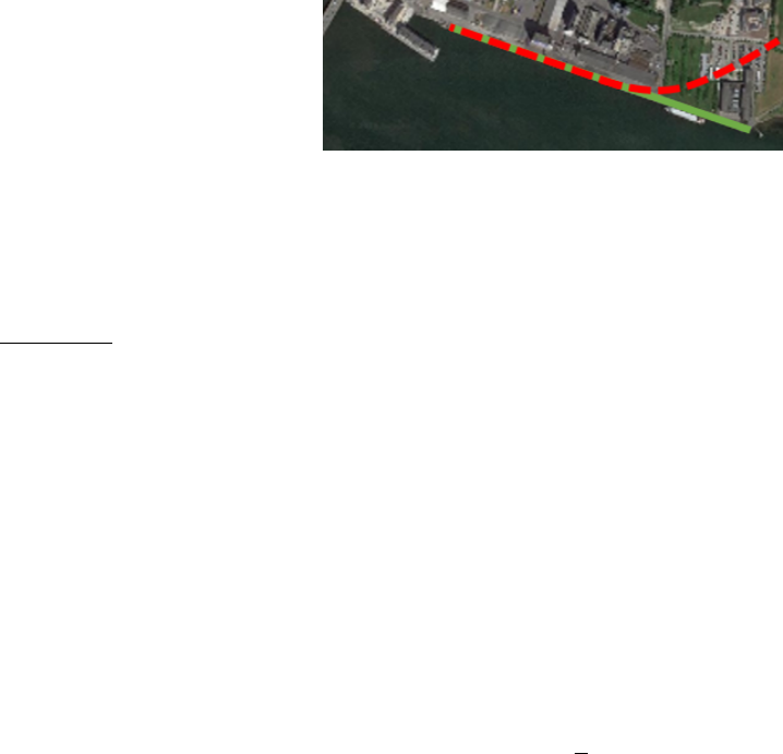
5.5 Calibration
The orientation of the camera was aligned with the
orientation of the map by offsetting the tilt and pan
of the camera. The estimated position of the wa-
terfront’s intersection with the waterline was tested.
This test showed that estimated position started to de-
viate from the true position as the camera was panned
to the right, illustrated in Figure 10. In this image
Figure 10: An illustration of a problem with the position
estimation when panning to the right. The dotted red line is
the position given by the estimator and the green line is the
actual position of the waterfront.
the green line indicates the line on which the posi-
tions should lie and the dotted red line illustrate where
they actually lay. This error was expected to be be-
cause of panoramic distortion which is a mechanical
effect which cause straight lines to curve as the cam-
era is panned (Luhmann, 2008). This expectation was
tested by creating a panoramic image of the water-
front which can be seen in Figure 11. In this image
the green line indicates the expected direction of the
waterfront if no distortion is present and the red dot-
ted line indicates the actual shape of the waterfront in
the images. The panoramic image was created manu-
ally by connecting images in succession and no other
manipulation of the images was performed. Compar-
ing Figure 10 and 11 the estimation error follows the
panoramic distortion well. The error was mitigated
by applying a function to the tilt based on a fraction
of the pan angle given by
t = t + (
p
f
), (3)
where t and p are tilt and pan respectively and f is the
fraction. The equation is only applied when the pan
angle is negative, i.e., where the camera is pointing
to the right, since this was the side that produced the
error. The fraction of the pan angle was found through
empirical tests.
5.6 Evaluation
In order to evaluate the position estimator, points rec-
ognizable in both the image and on the map were
used. This resulted in the points on the waterfront
shown in Figure 12, where the circles represent the

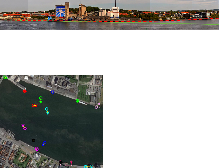
Figure 11: A panoramic image created of the waterfront. The dotted red line showing the waterfront as seen by the camera
and the green line indicating the expected shape of the waterfront provided no panoramic distortion.
chosen position, the stars represent the estimated po-
sition, and the colors indicate the connection between
points. The yellow line is added to clarify the con-
nection and show by how much they differ. Since
Figure 12: Position estimation test results. Circles represent
the true position. Stars and triangles represent the estimated
position.
the points which are recognizable in both the images
and on the map only lie on the edges of the water-
front, and not on the water, an additional test was per-
formed. In this test the position of a boat on the water
was estimated over time. Simultaneously the boat’s
GPS position was recorded from a boat tracking web-
site (MarineTraffic, 2019) which was used as ground
truth. The position of the boat detected by both sys-
tems is plotted in Figure 12 as the points on the water,
in which the triangles represent the estimated posi-
tion and the connected circles represent the position
from the tracking software. The mean and standard
deviation error of the position estimator for the points
on the waterfront where 12.54m and 11.49m respec-
tively, 25.63m and 21.30m for the tracked boat and,
18.58m and 19.87m when the two where combined.
The reason for the mean and standard deviation being
higher for the boat points. The reason for the mean
and standard deviation being higher for the boat posi-
tions is most likely due to the inaccuracy of the em-
bedded GPS systems which, by the International Mar-
itime Organization (IMO), are expected to be around
10 meters (IMO, 2001).
6 CONCLUSION
In this paper we present a method for monitoring
boat traffic in ports using computer vision. The
proposed method is divided into subsystems, which
were tested separately. The detection accuracy of
YOLOv3 was increased from an AP score of 75.58%
and 36.42% for optical and thermal images, respec-
tively, to 95.53% and 96.82% when fine-tuned with
just 450 annotated images. When testing models with
a dataset of images during low optical light conditions
the thermal model outperforms the optical model as
expected. The AP scores were 15.05% and 46.05%,
for the optical and thermal model, respectively. The
position estimation was evaluated to have a mean er-
ror between 12.54 m and 25.63 m depending on the
location of the estimated point. A large error was
generally experienced when estimating positions of
boats, which was most likely caused by inaccurate
GPS positions used as ground truth. Combining all
subsystems we have shown that boat traffic at ports
can be monitored by a single bi-spectrum camera. We
have shown that YOLOv3 can be retrained to detect
boats in optical and thermal images using a limited
amount of data. Lastly, we have shown that the posi-
tion of boats can be estimated using ray-casting.
6.1 Discussion
The boat detector is run twice: once for the opti-
cal image and once for the thermal. A solution that
would simplify and speed up the system would be to
incorporate early fusion, where the optical image and
thermal image are combined to create a 4-channel im-
age and run only a single instance of object detection.
However, that would require that the network is de-
signed for 4-channel images, and trained with a large
amount of 4-channel data. The test in low optical light
conditions should also be redone with a larger dataset
to get a better sense of the performance difference be-
tween the two detectors. Both models could likely

also be improved for detecting boats during low opti-
cal lighting conditions by training them with data cap-
tured in low optical lighting. The position estimator
could be improved by creating a better model for cor-
rection the panoramic distortion along with a better
calibration of the setup. A sensor constantly monitor-
ing the water level could also be implemented to more
precisely determine the cameras height above the wa-
ter. The position estimator should ideally be tested
using more accurate ground truth data. A tracking al-
gorithm could also be implemented for the purpose of
tracking the detected boats in the images. This would
ease the needed computations since the object detec-
tor would not need to be run for each frame. This
tracker could also provide more information such as
the path of certain boats and their velocity. An ad-
ditional advantage of tracking would be the ability to
automatically pan and tilt the camera to follow a spe-
cific boat. Classifying detected boats would be ben-
eficial in order to gain further statistical data about
the boats entering and leaving ports. This could be
done, provided enough data, by retraining both detec-
tion models to detect particular types of boats such as
sailboats, motorboats, and tankers.
REFERENCES
Agarwal, A., Jawahar, C. V., and Narayanan, P. J. (2005). A
survey of planar homography estimation techniques.
Technical report.
Akiyama, T., Kobayashi, Y., Kishigami, J., and Muto, K.
(2018). Cnn-based boat detection model for alert
system using surveillance video camera. In 2018
IEEE 7th Global Conference on Consumer Electron-
ics (GCCE), pages 669–670.
Branch, A. E. (1986). Port traffic control, pages 124–143.
Springer Netherlands, Dordrecht.
Chen, K., Pang, J., Wang, J., Xiong, Y., Li, X., Sun, S.,
Feng, W., Liu, Z., Shi, J., Ouyang, W., Loy, C. C.,
and Lin, D. (2019). Hybrid task cascade for instance
segmentation.
Council of the European Union (2008). Maritime surveil-
lance - overview of ongoing activities. Technical re-
port, European Union, Brussels.
Dalal, N. and Triggs, B. (2005). Histograms of oriented gra-
dients for human detection. In 2005 IEEE Computer
Society Conference on Computer Vision and Pattern
Recognition (CVPR’05), volume 1, pages 886–893
vol. 1.
Drawil, N., Amar, H., and Basir, O. (2013). Gps localization
accuracy classification: A context-based approach. In-
telligent Transportation Systems, IEEE Transactions
on, 14:262–273.
Gade, R. and Moeslund, T. (2014). Thermal cameras and
applications: A survey. Machine Vision and Applica-
tions, 25:245–262.
Girshick, R., Donahue, J., Darrell, T., and Malik, J. (2013).
Rich feature hierarchies for accurate object detection
and semantic segmentation.
Goshtasby, A. (1986). Piecewise linear mapping functions
for image registration. Pattern Recognition, 19(6):459
– 466.
Goshtasby, A. (1988). Image registration by local ap-
proximation methods. Image and Vision Computing,
6(4):255 – 261.
Hikvision (2019). Ds-2td4166-25(50). https://
www.hikvision.com/en/Products/Thermal-Camera/
Network-Speed-Dome/640512-Series/DS-2TD4166-
25(50).
Huang, J., Rathod, V., Chen, S., Zhu, M., Korattikara, A.,
Fathi, A., Fischer, I., Wojna, Z., Yang, S., Guadar-
rama, S., and Murphy, K. (2017). Speed/accuracy
trade-offs for modern convolutional object detectors.
Hughes, J. F., van Dam, A., McGuire, M., Sklar, D. F.,
Foley, J. D., Feiner, S. K., and Akeley, K. (2013).
Computer graphics: principles and practice (3rd ed.).
Addison-Wesley Professional, Boston, MA, USA.
IMO (2001). Guidelines for the onboard operational use
of shipborne automatic identification systems (ais).
page 6.
John, V., Tsuchizawa, S., Liu, Z., and Mita, S. (2016). Fu-
sion of thermal and visible cameras for the application
of pedestrian detection. Signal Image and Video Pro-
cessing.
Lin, T., Maire, M., Belongie, S. J., Bourdev, L. D., Girshick,
R. B., Hays, J., Perona, P., Ramanan, D., Doll
´
ar, P.,
and Zitnick, C. L. (2014). Microsoft COCO: common
objects in context. CoRR, abs/1405.0312.
Liu, L., Ouyang, W., Wang, X., Fieguth, P., Chen, J., Liu,
X., and Pietik
¨
ainen, M. (2018). Deep Learning for
Generic Object Detection: A Survey. arXiv e-prints,
page arXiv:1809.02165.
Liu, W., Anguelov, D., Erhan, D., Szegedy, C., Reed, S.,
Fu, C.-Y., and Berg, A. C. (2016). Ssd: Single shot
multibox detector. Lecture Notes in Computer Sci-
ence, page 21–37.
Luhmann, T. (2008). A historical review on panorama
photogrammetry. International Archives of the Pho-
togrammetry, Remote Sensing and Spatial Informa-
tion Sciences, 34.
MarineTraffic (2019). Marinetraffic: Global ship track-
ing intelligence — ais marine traffic. https://www.
marinetraffic.com/.
Mohan, D. and Ram, D. A. R. (2015). A review on depth es-
timation for computer vision applications. volume 4.
Redmon, J., Divvala, S., Girshick, R., and Farhadi, A.
(2016). You only look once: Unified, real-time ob-
ject detection. pages 779–788.
Redmon, J. and Farhadi, A. (2017). Yolo9000: Better,
faster, stronger. 2017 IEEE Conference on Computer
Vision and Pattern Recognition (CVPR), pages 6517–
6525.
Redmon, J. and Farhadi, A. (2018). Yolov3: An incremental
improvement. CoRR, abs/1804.02767.

Viola, P. and Jones, M. (2001). Rapid object detection us-
ing a boosted cascade of simple features. In Proceed-
ings of the 2001 IEEE Computer Society Conference
on Computer Vision and Pattern Recognition. CVPR
2001, volume 1, pages I–I.
Wiersma, E. and Mastenbroek, N. (1998). Measurement
of vessel traffic service operator performance. AI &
SOCIETY, 12(1):78–86.
Yosinski, J., Clune, J., Bengio, Y., and Lipson, H. (2014).
How transferable are features in deep neural networks.
CoRR, abs/1411.1792.
Zhang, E. and Zhang, Y. (2009). Average Precision, pages
192–193. Springer US, Boston, MA.
Zhang, Z. (2000). A flexible new technique for camera cal-
ibration. IEEE Transactions on Pattern Analysis and
Machine Intelligence, 22(11):1330–1334.
Zhu, R., Zhang, S., Wang, X., Wen, L., Shi, H., Bo, L.,
and Mei, T. (2018). Scratchdet: Training single-shot
object detectors from scratch.
Zou, Z., Shi, Z., Guo, Y., and Ye, J. (2019). Object detection
in 20 years: A survey. CoRR, abs/1905.05055.