
Low-density EEG for Source Activity Reconstruction using Partial Brain
Models
Andres Felipe Soler
1
, Eduardo Giraldo
2
and Marta Molinas
1
1
Department of Engineering Cybernetics, Norwegian University of Science and Technology, Trondheim, Norway
2
Department of Electrical Engineering, Universidad Tecnol
´
ogica de Pereira, Pereira, Colombia
Keywords:
Low-density EEG, Partial Brain Model, Source Reconstruction, Brain Mapping, EEG Signals.
Abstract:
Brain mapping studies have shown that the source reconstruction performs with high accuracy by using high-
density EEG montages, however, several EEG devices in the market provide low-density configurations and
thus source reconstruction is considered out of the scope of those devices. In this work, our aim is to use a few
numbers of electrodes to reconstruct the neural activity using partial brain models, therefore, we presented a
pipeline to estimate the brain activity using a low-density EEG on brain regions of interest, the partial brain
model formulation and several criteria for channel selection. Two regions have been considered to be studied,
the occipital region and motor cortex region. For the presented study synthetic EEG signals were generated
simulating the activation of sources with a frequency in the beta range at the occipital region, and mu rhythm
range at the motor cortex areas. Novel methods for electrode reduction and models for specific brain areas
are presented. We assessed the quality of the reconstructions by measuring the localization error, obtaining a
mean localization error below 7 mm and 16 mm with sLORETA and MSP methods respectively, by using a
low-density EEG with eight channels and partial brain models.
1 INTRODUCTION
Electroencephalography (EEG) is a non-invasive
technique that allows measuring the electrical brain
activity from the scalp with a high temporal resolu-
tion compared with other techniques like Functional
Magnetic Resonance Imaging (fMRI), Computed To-
mography (CT), and Positron Emission Tomography
(PET). Since the first report about brain activity mea-
sured by electrodes was presented by Hans Berger in
1924 (O’Leary, 1970), EEG technique has been used
to study various brain processes like memory and
emotions, brain diseases like Parkinson and epilepsy,
and human behavior, in attempts to understand the
complexity underlying processing capabilities of the
brain. Source analysis based on brain mapping tech-
niques are allowed to reconstruct the cortical activ-
ity from electrodes on the scalp solving the EEG
inverse problem. Several methods have been pro-
posed to provide a estimation of the neural activity,
like minimum norm estimation MNE (H
¨
am
¨
al
¨
ainen
and Ilmoniemi, 1994) or low-resolution tomography
LORETA (Pascual-Marqui et al., 1994).
In brain mapping research, it has been established
that a high number of electrodes is required to localize
accurately and reconstruct the cortical activity. How-
ever, a few studies have shown the possibility to apply
brain mapping methods using a small number of elec-
trodes. E.g, in (Jatoi and Kamel, 2018), the authors
proposed and evaluated the use of seven electrodes
to map the activity of the whole brain using several
brain mapping methods, obtaining a localization ac-
curacy around 15 mm using multiple sparse priors
method MSP (Friston et al., 2008). In (Soler et al.,
2019), a low-density approach to BCI was presented,
in which the occipital activity was mapped using MSP
and a partial brain model of the occipital region, ob-
taining an accuracy around 23 mm in the location of
the source with four electrodes using simulated activ-
ity, however, a channel selection criteria were not es-
tablished and the partial brain model was briefly for-
mulated.
The aim of this current study is to establish a
pipeline to apply low-density EEG configurations for
source activity reconstruction using partial brain mod-
els, presenting the formulation to map the brain based
on regions of interest. Additionally, several criteria
are proposed to perform a selection of the channels
to be used for brain mapping, two criteria are consid-
ered, one based on local electrodes around the target
54
Soler, A., Giraldo, E. and Molinas, M.
Low-density EEG for Source Activity Reconstruction using Partial Brain Models.
DOI: 10.5220/0008972500540063
In Proceedings of the 13th International Joint Conference on Biomedical Engineering Systems and Technologies (BIOSTEC 2020) - Volume 2: BIOIMAGING, pages 54-63
ISBN: 978-989-758-398-8; ISSN: 2184-4305
Copyright
c
2022 by SCITEPRESS – Science and Technology Publications, Lda. All rights reserved

zone, and a second one based on a relevance crite-
rion. In this work, we presented a pipeline to esti-
mate the brain activity, to test our methodology, we
used synthetic EEG signals, simulating sources over
two brain regions, the occipital region, and motor cor-
tex region. We use the localization error to evaluate
the reconstructions comparing the position of the es-
timated sources versus the simulated one.
2 MATERIAL AND METHODS
2.1 Forward EEG Model
The relation between the EEG electrodes distributed
on the scalp and the source activity can be represented
by the forward problem equation:
y
y
y = M
M
Mx
x
x + ε (1)
where M
M
M ∈ R
d×n
represents the volume conductor
model, also known by leadfield matrix. This matrix
represents the conductivity of the brain and explains
how the potentials flow through brain from a set of
n distributed sources to d number of electrodes on
the scalp. This volume conductor model in realis-
tic brain representations considers the head anatomy
and the conductivity of the different tissues and lay-
ers between current sources and electrodes, like white
matter, gray matter, CSF, skull and scalp (Vorwerk
et al., 2012; Huang et al., 2016). y
y
y ∈ R
d×k
represents
the signals recorded by the electrodes in k number
of samples, the source activity matrix is represented
by x
x
x ∈ R
n×k
, it contains the amplitude of distributed
sources over the brain cortical areas. ε represents the
noise covariance, and it is assumed to follow a normal
distribution with zero mean.
2.2 Partial Brain Model Formulation
Consider the problem of EEG generation for a time
instant given by the forward EEG equation in 1. This
model can be rewritten by considering two subsets of
brain activity x
x
x as follows:
y
y
y =
M
M
M
1
M
M
M
2
x
x
x
1
x
x
x
2
+ ε
ε
ε (2)
being M
M
M
1
and x
x
x
1
being the leadfield matrix and its
corresponding neural activity for a specific brain zone
of interest or target zone, and M
M
M
2
and x
x
x
2
the lead-
field matrix and its corresponding neural activity of
the remaining brain. It can be seen that the (2) can be
rewritten as
y
y
y = M
M
M
1
x
x
x
1
+ η
η
η (3)
η
η
η being a vector that holds the noise and the activity
in the part of the brain related to M
M
M
2
and x
x
x
2
. In addi-
tion, if the vector x
x
x
2
is close to zero (which means that
the neural activity outside the target zone is closed to
zero), the following approximation can be performed
y
y
y ≈ M
M
M
1
x
x
x
1
+ ε
ε
ε (4)
By using an approximated model as described in
(4) the inverse problem for
ˆ
x
x
x
1
can be solved. How-
ever, the activity outside the target zone could affect
the estimation because all the recorded activity by the
electrodes will be projected in the target zone. There-
fore, an additional stage to reduce the effect of M
M
M
2
x
x
x
2
over y
y
y can be added before performing the inverse
problem, by considering that the source in the target
zone appears in a known frequency, then, the EEG
is filtered using band-pass filters leading to an atten-
uation of the activity outside the region of interest.
In addition, by assuming that the electrodes mostly
record activity in the neighbor spaces around it, a re-
duction in the number of electrodes can be made as
y
y
y
r
≈ M
M
M
1r
x
x
x
1r
+ ε
ε
ε
r
(5)
where the resulting estimation of x
x
x
1r
is an approxi-
mation of x
x
x
1
obtained by using a reduced number of
channels.
A partial brain model is a section of the brain
based on a specific zone of interest and it is gener-
ated from a complete brain model. For that purpose,
we used the brain model denominated as the New
York Head (ICBM-NY) presented in (Huang et al.,
2016), this is based on the computation of a finite ele-
ment method (FEM) over a non-linear average of 152
individual MRI (ICBM152 v2009) from the Interna-
tional Consortium for Brain Mapping (Fonov et al.,
2009). The New York Head was calculated consider-
ing the conductivity of six tissue types: scalp, skull,
CSF, gray matter, white matter and air cavities with
a resolution of 0.5mm
3
. The lead field matrix of the
New York Head was calculated for 74382 distributed
sources and 231 electrodes, however, several strict
subsets of sources with 10016, 5008 and 2004 vertices
are available at https://www.parralab.org/nyhead/.
We selected the model of 10016 and performed
an electrode reduction to 60 positions of the 10-20
international system (Fig.1A), this model is referred
to the paper as 10K model and it is used to compare
the performance of a high-density montage versus the
partial brain models with low-density EEG.
We generated a partial brain model of two brain
areas: occipital cortex area (Fig.1B) referred to OC
model, and the motor cortex area referred to MC
model (Fig.1C). The number of distributed sources
for the partial brain models is 3054 for the OC model
and 2162 for the MC model.
Low-density EEG for Source Activity Reconstruction using Partial Brain Models
55
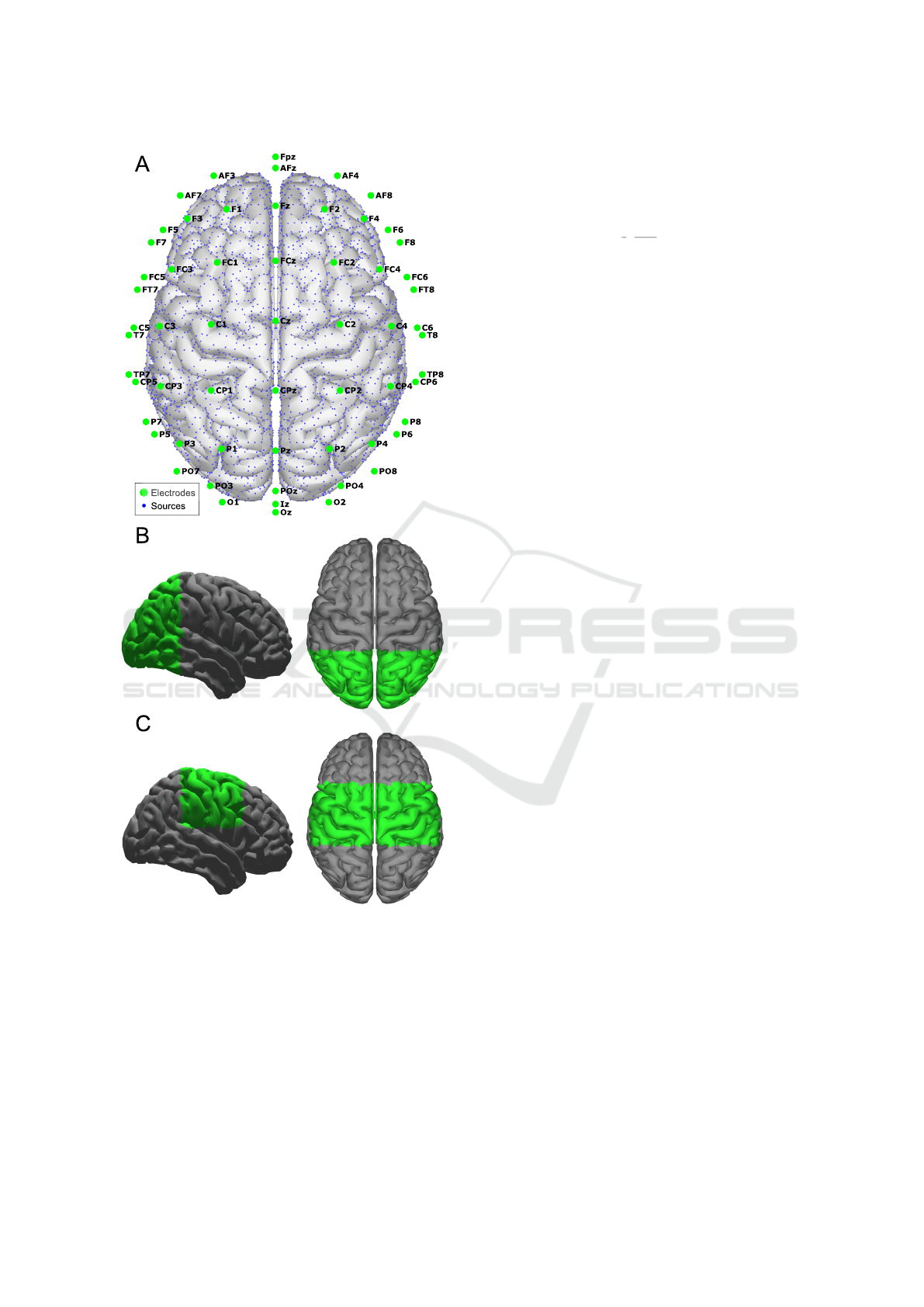
Figure 1: Head model with 60 electrodes and 10016
sources, 10K model (A), Brain section for occipital cortex
area partial brain model, OC model (B), and Brain section
for motor cortex area partial brain model, MC model (C).
2.3 Synthetic EEG Generation
With the purpose to evaluate the performance of the
partial brain models for source reconstruction, we
generated 400 trials of simulated EEG activity at five
levels of noise: 0, 5, 10, 15, and 20dB (80 trials per
level). Each trial has two simulated sources over-
lapping between 37.5% and 40% . Each simulated
source activity was computed using a windowed si-
nusoidal activity using the following equation:
x
i
(t
k
) = e
−
1
2
(
t
k
−c
i
σ
)
2
sin(2π f
i
t
k
) (6)
where σ = 0.12 determines the Gaussian window
width. The first source s
1
was simulated in the oc-
cipital areas, with a frequency f
1
of 20Hz (simulating
a source in the range of Beta wave), and centered at
c
1
= 300ms. The second source s
2
was simulated in
the motor cortex areas, with a frequency f
2
of 10Hz
(simulating a source in the range of mu rhythm), and
centered at c
2
= 800ms. The positions were randomly
selected between a set of pre-defined positions dis-
tributed on the corresponding target zone. The pre-
defined set of positions has six locations, three in each
hemisphere, the positions were: 3727, 8735, 2734,
7742, 3461, and 8469 for the source s
1
at occipital ar-
eas and 3837, 8845, 2284, 7292, 2271, and 7279 for
the source s
2
at motor cortex areas. An example of the
simulated activity is shown in Fig.2. It shows the lo-
cation of the simulated sources at the center of activity
and the time courses of the sources during the simu-
lated trial, in addition, the EEG related to the simu-
lated activity is presented with the electrodes labeling.
2.4 Channel Selection
We applied two criteria to select the electrodes: us-
ing local electrodes around the region of interest as
presented in (Soler et al., 2019), and using a channel
relevance analysis applying the Q-α method proposed
by (Wolf and Shashua, 2005). Those criteria are ex-
plained below:
2.4.1 Local Electrodes
The concept of local electrodes is based on the hy-
pothesis that the electrodes mostly record the electri-
cal activity of the near space around it. To select an
electrode configuration we considered the results of
the previous work of (Soler et al., 2019), in which
a four-electrode configuration was used to map one
source in the occipital region with a mean localiza-
tion error of 23 mm. Therefore, to evaluate the con-
cept of local electrodes and compare if increasing the
number of electrodes decreases the error, we selected
a configuration of eighth electrodes around the tar-
get zone, maintaining an equal number of electrodes
across both brain hemispheres. Those configurations
are shown in Fig.3 for the OC and MC partial brain
models.
BIOIMAGING 2020 - 7th International Conference on Bioimaging
56
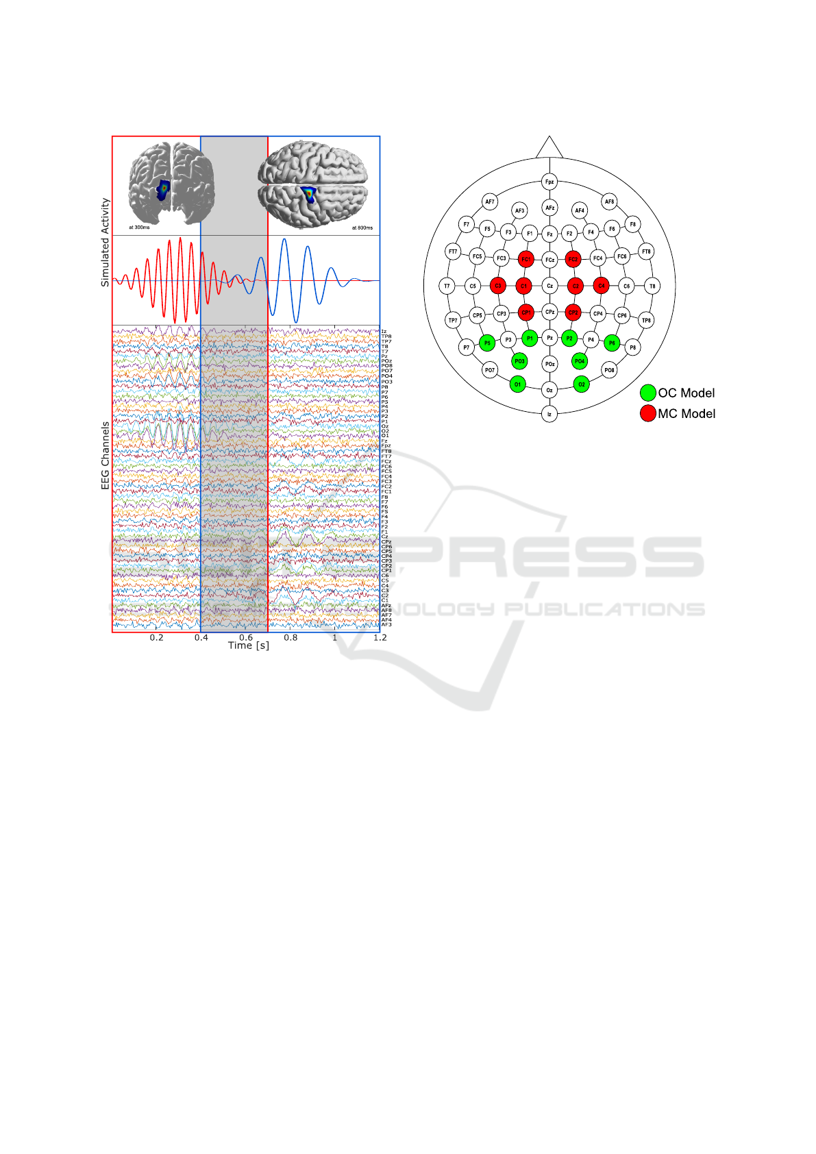
Figure 2: Example of source activity (top), source activ-
ity one simulated between 0-0.7s at 20Hz in the occipital
area (red), source activity two simulated between 0.4-1.2s
at 12Hz in the motor cortex (blue). EEG and channel infor-
mation (bottom). The overlap between the source activity
one and two is around a 37.5% to 42% (marked in the gray
area).
2.4.2 Relevance Analysis
We performed a relevance analysis based on the Q-α
method, applying the Standard Power-Embedded Q-α
algorithm. This method was originally proposed for
feature selection in unsupervised and supervised in-
ference problems (Wolf and Shashua, 2005; Wolf and
Shashua, 2003), in which a set of features is weighted
with an α vector coefficient according to the cluster-
ing quality of data points. Under this approach, let
define the EEG data y
y
y as the data points matrix with
k samples, and each row correspond to an electrode
containing the voltage information of a specific loca-
tion as a feature to weight. Each electrode denoted
Figure 3: Electrode layout and selected local electrodes, lo-
cal electrodes for OC partial brain model (green), and local
electrodes for MC partial brain model (red).
by y
y
y
T
1
, ..., y
y
y
T
k
is pre-processed such that each electrode
is centered around zero and its L
2
norm equal to one
(||y
y
y
i
|| = 1). Let define a vector α
α
α ∈ R
d
, which con-
tains the weight value associated with each electrode,
being α
α
α = (α
α
α
1
, ..., α
α
α
d
)
T
. Let A
A
A
α
be the correspond-
ing affinity matrix defined as A
A
A
α
=
∑
d
i=1
α
α
α
i
y
y
y
i
y
y
y
T
i
and
Q
Q
Q ∈ R
k×m
whose columns are the first m eigenvec-
tors of A
A
A
α
associated with the highest eigenvalues
λ
1
≥ ... ≥ λ
m
. The values of α
α
α and Q
Q
Q are unknown
and they can be calculated solving the following opti-
mization problem:
maxtrace
Q
Q
Q,α
α
α
(Q
Q
Q
T
A
A
A
T
α
A
A
A
α
Q
Q
Q)
subject to α
α
α
T
α
α
α = 1, Q
Q
Q
T
Q
Q
Q = I
(7)
by applying the Standard Power-Embedded Q-α
algorithm to solve the optimization problem, the α
α
α
weights are calculated. This method was applied be-
fore in a source reconstruction setting to weight the
electrodes in an inverse problem solution algorithm
presented by (Giraldo et al., 2012). In contrast, our
proposed approach is to select a set of channels with
the highest weights to perform the brain source recon-
struction using the partial brain models. We defined
three levels of relevance, based on the 4, 8 and 16
most relevant electrodes.
2.5 Brain Source Reconstruction
The source reconstruction is an estimation of the cor-
tical activity using the registered voltages by elec-
Low-density EEG for Source Activity Reconstruction using Partial Brain Models
57

trodes on the scalp. To estimate the neural activity
in cortical regions, the EEG inverse problem must
be solved. This problem is considered ill-posed and
ill-conditioned due to the information available on
the scalp, which is limited to hundreds of electrodes,
while, the number of unknowns or sources to estimate
is in the order of thousands.
Several methods provide a solution for the elec-
tromagnetic inverse problem based on electrodes in-
formation and the model of the conductivity. We se-
lected two methods for brain mapping: the standard-
ized low-resolution tomography sLORETA (Pascual-
Marqui, 2002), and multiple sparse priors MSP (Fris-
ton et al., 2008). sLORETA was selected due to the
low localization error presented by its author, even in
some cases, zero error localization(Jatoi et al., 2014).
On the other hand, MSP has been tested with low-
density EEG montages by (Jatoi and Kamel, 2018)
and has shown lower localization error than other
methods like minimum norm estimation MNE and
LORETA (L
´
opez et al., 2014).
The MSP implementation used is a freely avail-
able software package SPM12 (Wellcome Trust Cen-
tre for Neuroimaging), we set up the number of
patches to 1100 according to the findings using seven
electrodes in (Jatoi and Kamel, 2018). The method
sLORETA was implemented based on the code pro-
vided in by (Biscay et al., 2018).
2.6 Pipeline
The followed pipeline is summarized in Fig.4A. The
procedure started with the simulation of the neural ac-
tivity using Eq.6, two sources s
1
and s
2
were simu-
lated. To generate the EEG signals, the activity matrix
x is created and the sources were located in random
positions, s
1
in occipital areas and s
2
in motor cortex
areas, none of the sources was located outside the tar-
get to avoid a projection of an external source in the
partial brain model. With the computed source activ-
ity x, and using the 10K model, the forward problem
was calculated applying the Eq.1, the estimated EEG
was contaminated with noise at five levels of signal-
noise-ratio SNR of 0, 5, 10, 15, and 20dB. For detailed
information of the EEG generation we refer to section
2.3.
Each EEG trial is filtered by using a high order
FIR band-pass filters, the cutoff frequencies were set
up at 19 and 21Hz for the first source s
1
, and for the
second source s
2
were at 9 and 11Hz. The filters were
applied in both direction of time to prevent losing in-
formation. As the output of the filter stage, two fil-
tered set of EEG signals were obtained y
y
y
s
1
and y
y
y
s
2
for
the respective simulated source.
After filtering, several EEG reductions were cal-
culated according to the channel selection criteria,
y
y
y
s
1
loe
and y
y
y
s
2
loe
by the local channel criterion,
y
y
y
s
1
rel4e
and y
y
y
s
2
rel4e
by the first level of relevance with
four electrodes, y
y
y
s
1
rel8e
and y
y
y
s
2
rel8e
by the second
level of relevance with eight electrodes, and y
y
y
s
1
rel16e
and y
y
y
s
2
rel16e
by the third level of relevance with 16
electrodes.
The source reconstruction was performed with
both methods MSP and sLORETA over all the ten
EEG data, therefore, 20 source reconstructions were
computed, four using the high-density montage with
60 electrodes and the 10K model, eight applying the
channel selection criteria and the OC model, and
eight applying the channel selection criteria and the
MC model. A diagram with the name of each EEG
data and the respective reconstructions is presented in
Fig.4B.
Finally, the localization error was calculated com-
paring the resulting source position versus the original
simulated position, using the following equation:
LocE = ||
ˆ
P
x
− P
ˆx
||
2
(8)
where P
x
is the position in a 3D coordinated space
of the simulated activity and P
ˆx
the position of the
maximum amplitude source of the estimated activity.
To provide a view of the effects of filtering, the
same 20 reconstructions were calculated eliminating
the filtering stage from the pipeline, making y
y
y
s
1
and
y
y
y
s
2
equal to y
y
y, however, the same respective models
were used to perform the source reconstruction stage.
Because the source s
1
has higher mean power than
s
2
due to the higher frequency, we were interested in
evaluating the performance of the channel selection
criteria and the brain mapping methods without iso-
lating the sources using the filtering process.
3 RESULTS
A general view of the results is provided in Fig.5. At
the top, the mean localization errors of the source
reconstructions are presented, they were calculated
eliminating the filtering stage from the pipeline. In
contrast, at the bottom, the mean localization errors
of the source reconstructions are presented using the
complete pipeline. Additionally, the results are sum-
marized in Table 1.
In a general point of view regarding the effects of
filtering, when the filter stage was not applied (Fig.
5A and Table 1), the sources were mixed and the rel-
evance criteria tended to select the channels related to
the highest power source, in the case of the source s
1
,
BIOIMAGING 2020 - 7th International Conference on Bioimaging
58
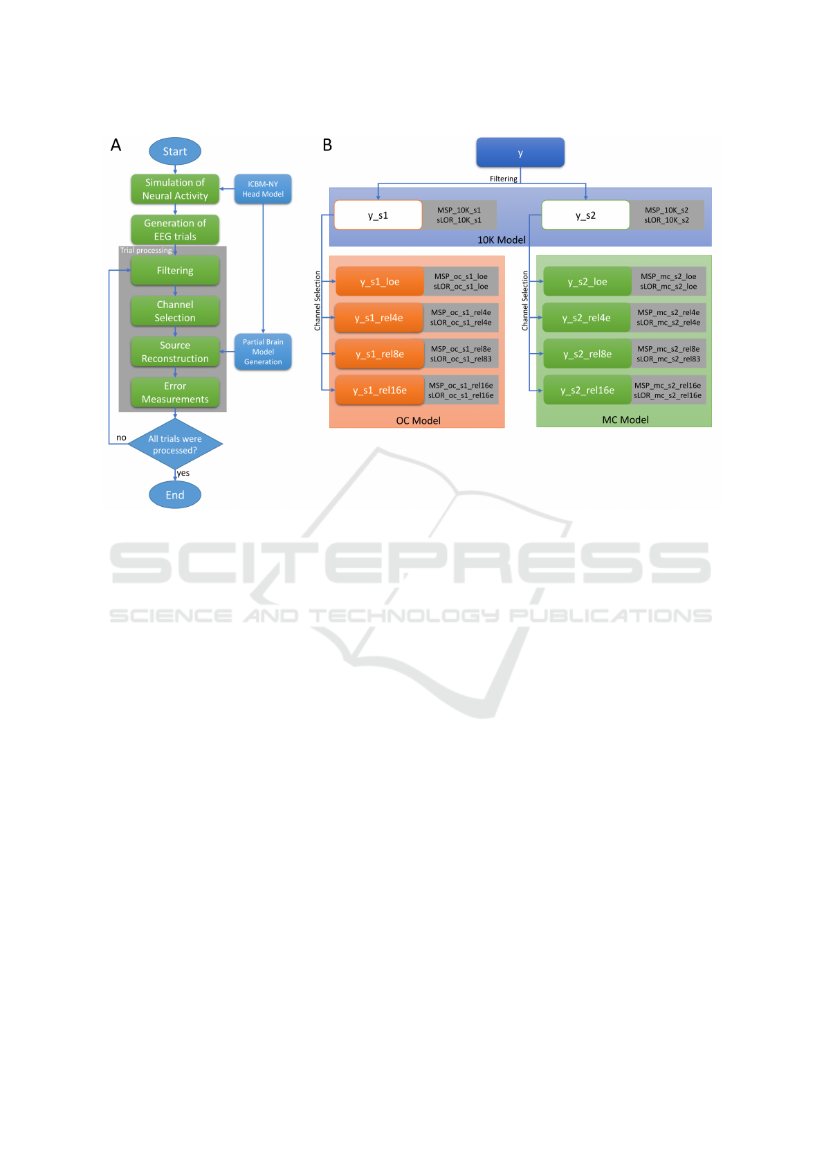
Figure 4: The flowchart of the followed pipeline (A), after the trial generation, the procedure is applied per trial (gray square).
Source reconstruction tree (B), gray squares contain the name of the reconstruction using the EEG signal at left, the region in
blue indicates the use of the 10K model, orange for the OC model, and green for the MC model.
due to the high frequency, it presents a higher power
than source s
2
, therefore it was reconstructed with
higher accuracy than s
2
. The accuracy obtained with-
out filtering for the source s
2
shows that the methods
projected the s
1
in the MC model, which explains the
high mean localization error of the methods using the
full set of electrodes. By inspection of the selected
electrodes using the relevance criteria, in most of the
cases, the electrodes were near to the source s
1
due to
the lack of isolation by bypassing the filtering stage.
The best reconstructions were obtained by the full
set of electrodes and the 10K model with filtering
and without filtering for the sLORETA, in the case
of MSP, the error increased significantly from 4 to
24 mm removing the filtering stage. Regarding the
reconstructions using the presented pipeline and the
partial brain models, the relevance channel selection
with 16 electrodes obtained the lowest localization er-
ror for both sources, followed by the second level of
relevance with 8 electrodes, the first level with 4 elec-
trodes, and finally, the eight local electrodes. In all
the cases the MSP method presented a low accuracy
than sLORETA.
The local electrodes criteria presented a stable
value for the reconstruction even if the filtering stage
was not applied. For the source s
1
with OC model, the
mean localization error was between 15 to 20 mm,
and for source s
2
and MC model, between 11 to 22
mm. In general, when used the partial brain models
and the channel selection by relevance, the localiza-
tion error remained below 10 mm for the sLORETA
method, and below 21 mm for the MSP reconstruc-
tions.
4 DISCUSSION
In this paper, we have presented a pipeline to recon-
struct the source activity over specific brain regions
using partial brain models and low-density EEG, us-
ing channel selection criteria.
In the presented simulations, we evaluated the per-
formance of partial brain models and the relevance
analysis for channel selection, the results showed by
using of sLORETA the mean localization error were
below 10mm, which in several cases is even low than
localization error values obtained by other methods
with high-density montages as explained in several
works by (L
´
opez et al., 2014; Jatoi and Kamel, 2018).
Comparing to (L
´
opez et al., 2014), we obtained a
similar error value around 5 mm for our high-density
montage with MSP.
The use of partial brain models constraint the
Low-density EEG for Source Activity Reconstruction using Partial Brain Models
59
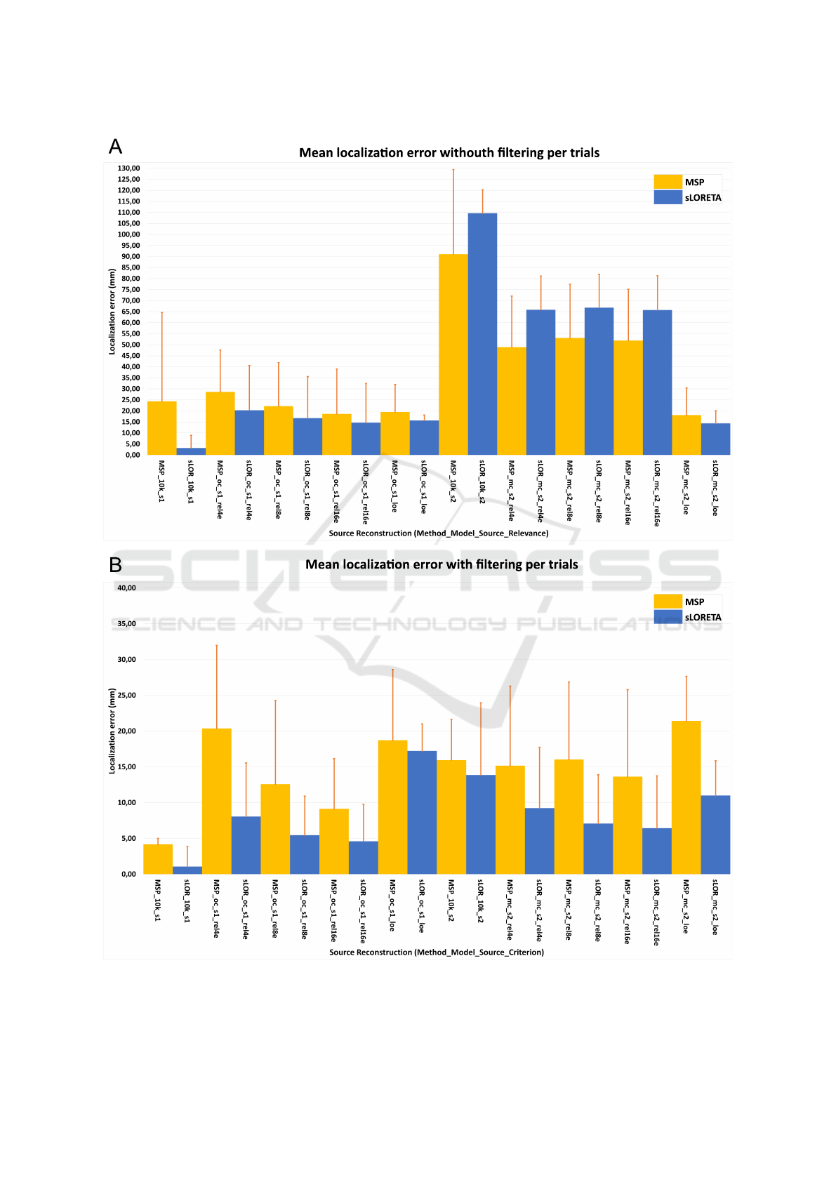
Figure 5: Mean error localization, without applying the filter stage (A), and following the complete pipeline with the filtering
stage (B).
BIOIMAGING 2020 - 7th International Conference on Bioimaging
60

Table 1: Mean error localization without applying the filter stage, and following the complete pipeline including the filtering
stage.
Non-Filtered Data Filtered Data
Method
Head
Model
Source
Channel
Selection
Criteria
Number
of
Electrodes
Mean
Localization
Error (mm)
SD
Mean
Localization
Error (mm)
SD
MSP 10K S1 - 60 24,41 40,22 4,19 0,82
sLORETA 10K S1 - 60 3,22 5,70 1,08 2,79
MSP OC S1 Relevance 4 28,67 18,97 20,37 11,63
sLORETA OC S1 Relevance 4 20,33 20,26 8,07 7,48
MSP OC S1 Relevance 8 22,19 19,69 12,58 11,72
sLORETA OC S1 Relevance 8 16,74 18,86 5,46 5,46
MSP OC S1 Relevance 16 18,68 20,29 9,14 7,02
sLORETA OC S1 Relevance 16 14,67 17,74 4,61 5,17
MSP OC S1 Local 8 19,47 12,54 18,73 9,89
sLORETA OC S1 Local 8 15,70 2,44 17,23 3,79
MSP 10K S2 - 60 91,09 38,32 15,94 5,71
sLORETA 10K S2 - 60 109,66 10,61 13,87 10,08
MSP MC S2 Relevance 4 48,90 23,16 15,17 11,13
sLORETA MC S2 Relevance 4 65,88 15,25 9,24 8,51
MSP MC S2 Relevance 8 53,09 24,39 16,05 10,82
sLORETA MC S2 Relevance 8 66,83 15,07 7,09 6,82
MSP MC S2 Relevance 16 51,93 23,19 13,64 12,17
sLORETA MC S2 Relevance 16 65,71 15,61 6,44 7,30
MSP MC S2 Local 8 18,14 12,27 21,44 6,22
sLORETA MC S2 Local 8 14,34 5,71 11,01 4,85
brain mapping methods to find a solution in a pre-
defined space, which will make it prone to error when
the source of interest originates from other areas. For
this reason, the application of partial brain models
should be restricted to applications in which the area
of interest that will be activated is well known, i.e,
in some visual evoked potentials VEP experiments
in which the interest is to know how the visual cor-
tex areas respond to certain stimuli (Vilhelmsen et al.,
2019; Van Der Meer et al., 2013), or in motor imagi-
nary task were is well known that the motor cortex is
activated (Burianov
´
a et al., 2013; Qiu et al., 2017).
Even if the results shown that the localization er-
ror was higher with the local electrodes than applying
the relevance criteria, this method can be applied in
settings in which a high quantity of electrodes is not
available. In addition, we consider that the use of lo-
cal electrodes can be applied in settings for which the
frequency of the source of interest is not well known.
As shown in Fig.5 and Table 1, the mean error was
kept below 22 mm regardless of the use of filters to
isolate the sources.
It is clear, regardless of the use of the filtering
stage, that the best reconstructions were obtained by
the full set of electrodes. However, its noticeable that
with the presented pipeline using low-density EEG
montages and the proposed partial brain models, we
achieved with eight electrodes a mean localization er-
ror around 7 mm with sLORETA and 16 mm with
MSP, and slightly less with 16 electrodes, around 6
mm with sLORETA and 14 mm with MSP.
5 CONCLUSIONS
In this work, we presented a formal definition of the
partial brain models and tested the capability to map-
ping a target zone of the brain using a reduced model
of a region of interest. We presented a pipeline to
apply those models and performed experiments with
multiple synthetic EEG trials with two overlapped
sources at several levels of noise and several levels of
electrode resolution based on channel selection cri-
teria. We measured the quality of the source recon-
structions with the localization error, and based on
the accuracy of the results obtained herein, we con-
sider that partial brain models following the pipeline
can reconstruct the source activity using low-density
EEG montages of 8 and 16 electrodes with a precision
below 10 mm with sLORETA and 20 mm with MSP.
As presented, we focused on the localization error
obtained with sLORETA and MSP for brain source
Low-density EEG for Source Activity Reconstruction using Partial Brain Models
61

reconstruction, however, it is worth noticing that the
solutions by sLORETA are smooth (Pascual-Marqui,
2002), while the other hand, MSP present more sparse
solutions (L
´
opez et al., 2014; Friston et al., 2008).
Therefore in future works, we will consider the use
of error measurements that involve the temporal evo-
lution of the reconstructed sources and the sparseness
of the solutions.
The pipeline presented considers a basic filter
stage using band-pass filters with the intention to fo-
cus on the partial brain models to source activity
reconstruction. However, several studies (Mu
˜
noz-
Guti
´
errez et al., 2018; Hansen et al., 2019) have
shown that the using of advanced techniques for fre-
quency decomposition like empirical mode decompo-
sition EMD, multivariate EMD, noise assisted EMD,
and wavelets can offer a solution for unmixing the
source activity improving the brain mapping algo-
rithms. Those techniques will be studied on partial
brain models in future publications.
AUTHOR CONTRIBUTIONS
This part was intentionally removed for reviewing
purposes All the authors conceived and designed the
experiments. AFS performed the experiments. All
the authors analyzed the data, wrote and refined the
article.
ACKNOWLEDGMENT
This part was intentionally removed for reviewing
purposes This work was supported by the Norwegian
University of Science and Technology NTNU, project
”David and Goliath: single-channel EEG unravels its
power through adaptive signal analysis”.
REFERENCES
Biscay, R. J., Bosch-Bayard, J. F., and Pascual-Marqui,
R. D. (2018). Unmixing EEG Inverse solutions based
on brain segmentation. Frontiers in Neuroscience,
12(MAY).
Burianov
´
a, H., Marstaller, L., Sowman, P., Tesan, G., Rich,
A. N., Williams, M., Savage, G., and Johnson, B. W.
(2013). Multimodal functional imaging of motor im-
agery using a novel paradigm. NeuroImage.
Fonov, V., Evans, A., McKinstry, R., Almli, C., and
Collins, D. (2009). Unbiased nonlinear average age-
appropriate brain templates from birth to adulthood.
NeuroImage, 47:S102.
Friston, K., Harrison, L., Daunizeau, J., Kiebel, S., Phillips,
C., Trujillo-Barreto, N., Henson, R., Flandin, G., and
Mattout, J. (2008). Multiple sparse priors for the
M/EEG inverse problem. NeuroImage, 39(3):1104–
1120.
Giraldo, E., Peluffo-Ordo
˜
nez, D., and Castellanos-
Dominguez, G. (2012). Weighted Time Series Analy-
sis for Electroencephalographic Source Localization.
DYNA Universidad Nacional de Colombia, 79:64–70.
H
¨
am
¨
al
¨
ainen, M. S. and Ilmoniemi, R. J. (1994). Interpret-
ing magnetic fields of the brain: minimum norm esti-
mates. Medical & Biological Engineering & Comput-
ing, 32(1):35–42.
Hansen, S. T., Hemakom, A., Gylling Safeldt, M., Krohne,
L. K., Madsen, K. H., Siebner, H. R., Mandic, D. P.,
and Hansen, L. K. (2019). Unmixing oscillatory
brain activity by EEG source localization and empiri-
cal mode decomposition. Computational Intelligence
and Neuroscience, 2019.
Huang, Y., Parra, L. C., and Haufe, S. (2016). The new
york head—a precise standardized volume conduc-
tor model for eeg source localization and tes target-
ing. NeuroImage, 140:150 – 162. Transcranial electric
stimulation (tES) and Neuroimaging.
Jatoi, M. A. and Kamel, N. (2018). Brain source localiza-
tion using reduced eeg sensors. Signal, Image and
Video Processing, 12(8):1447–1454.
Jatoi, M. A., Kamel, N., Malik, A. S., Faye, I., and Be-
gum, T. (2014). A survey of methods used for source
localization using eeg signals. Biomedical Signal Pro-
cessing and Control, 11:42 – 52.
L
´
opez, J. D., Litvak, V., Espinosa, J. J., Friston, K., and
Barnes, G. R. (2014). Algorithmic procedures for
Bayesian MEG/EEG source reconstruction in SPM.
NeuroImage, 84:476–487.
Mu
˜
noz-Guti
´
errez, P. A., Giraldo, E., Bueno-L
´
opez, M.,
and Molinas, M. (2018). Localization of active brain
sources from EEG signals using empirical mode de-
composition: a comparative study. Frontiers in Inte-
grative Neuroscience, 12.
O’Leary, J. (1970). Hans berger on the electroencephalo-
gram of man. the fourteen original reports on the hu-
man electroencephalogram. translated from the ger-
man and edited by pierre gloor. Science, 168:562–563.
Pascual-Marqui, R. D. (2002). Standardized low-resolution
brain electromagnetic tomography (sLORETA): Tech-
nical details. Methods and Findings in Experimental
and Clinical Pharmacology, 24(SUPPL. D):5–12.
Pascual-Marqui, R. D., Michel, C., and Lehmann, D.
(1994). Low resolution electromagnetic tomography:
a new method for localizing electrical activity in the
brain. International Journal of Psychophysiology,
18(1):49–65.
Qiu, Z., Allison, B. Z., Jin, J., Zhang, Y., Wang, X., Li, W.,
and Cichocki, A. (2017). Optimized motor imagery
paradigm based on imagining Chinese characters writ-
ing movement. IEEE Transactions on Neural Systems
and Rehabilitation Engineering, 25(7):1009–1017.
Soler, A., Giraldo, E., and Molinas, M. (2019). Partial Brain
Model For Real-Time Classification Of RGB Visual
BIOIMAGING 2020 - 7th International Conference on Bioimaging
62

Stimuli: A Brain Mapping Approach To BCI. In 8th
Graz Brain Computer Interface Conference.
Van Der Meer, A. L., Svantesson, M., and Van Der Weel,
F. R. (2013). Longitudinal study of looming in infants
with high-density EEG. Developmental Neuroscience,
34(6):488–501.
Vilhelmsen, K., Agyei, S. B., van der Weel, F. R., and
van der Meer, A. L. (2019). A high-density EEG
study of differentiation between two speeds and di-
rections of simulated optic flow in adults and infants.
Psychophysiology, 56(1).
Vorwerk, J., Clerc, M., Burger, M., and Wolters, C. H.
(2012). Comparison of boundary element and fi-
nite element approaches to the EEG forward problem.
Biomedizinische Technik, 57:795–798.
Wolf, L. and Shashua, A. (2003). Feature selection for un-
supervised and supervised inference: The emergence
of sparsity in a weighted-based approach. In Proceed-
ings of the IEEE International Conference on Com-
puter Vision, volume 1, pages 378–384.
Wolf, L. and Shashua, A. (2005). Feature Selection for
Unsupervised and Supervised Inference: The Emer-
gence of Sparsity in a Weight-Based Approach * Am-
non Shashua. Journal of Machine Learning Research,
6:1855–1887.
Low-density EEG for Source Activity Reconstruction using Partial Brain Models
63
