An Approximate Method for Integrated

Stochastic Replenishment Planning with Supplier Selection

Rabin Kumar Sahu

1,2 a

, Clarisse Dhaenens

2 b

, Nadarajen Veerapen

2 c

and Manuel Davy

Vekia, Euratechnologies-B

atiment Urbawood, 58 All

ee Marie-Th

ese Vicot-Lhermitte, F-59000 Lille, France

Universit

e de Lille, CNRS, Centrale Lille, UMR 9189 - CRIStAL - Centre de Recherche en Informatique Signal et

Automatique de Lille, F-59000 Lille, France

Keywords:

Stochastic Demand, Supplier Selection, Replenishment Planning, Heuristic, Integrated Planning.

Abstract:

A practical methodology for integrated stochastic replenishment planning with supplier selection is proposed

for the single item inventory system. A rolling horizon strategy is adopted to implement the ordering decisions.

Our method works in two stages. The ﬁrst stage is a general black box stage that gives the minimum expected

“coverage period” cost. The second stage uses a dynamic programming approach to compute the minimum

expected cost for the rolling horizon. The proposed method is applicable for both stationary and non-stationary

demand distributions and even for problems with minimum order quantity constraints. We also propose to

examine the beneﬁts of a dynamic supplier selection approach in comparison to selecting a common supplier.

We conduct extensive numerical analyses on synthetic data sets for validation.

1 INTRODUCTION

Integrated replenishment planning with supplier se-

lection is one of the core problems faced by retailers.

With growing competitiveness in the current market,

inclusion of purchasing price and thereby supplier se-

lection in inventory optimization becomes very im-

portant. The inherent multi stage stochastic pro-

gramming (MSSP) (Homem-de Mello and Bayrak-

san, 2014) problem for the multi-period inventory op-

timization problem is very difﬁcult to solve optimally

due to the well known curse of dimensionality (De-

fourny et al., 2012). Supplier selection adds addi-

tional decision or action states and further increases

the complexity. In this paper, we ﬁrst analyze the eco-

nomic beneﬁts of dynamic supplier selection and af-

terwards develop an approximate method to solve this

problem.

Supplier selection has received considerable atten-

tion in the inventory optimization literature post 2003.

Initially, supplier selection or multiple sourcing op-

tions have been seen as a measure of supply chain risk

mitigation. However, in addition to that, multiple sup-

pliers can have signiﬁcant monetary beneﬁts in terms

of costs. Most of the replenishment planning models

https://orcid.org/0000-0003-1597-6324

https://orcid.org/0000-0002-6590-7215

https://orcid.org/0000-0003-3699-1080

with multiple suppliers optimize the total cost. This

cost is the summation of the replenishment costs, in-

ventory holding costs and shortage costs. Replenish-

ment costs consist of purchasing cost of the item, and

ﬁxed order/setup costs for placing an order. Typically,

the ﬁxed order cost is independent of order quantity

and charged for every order placed. The purchasing

cost can be different for each supplier and inﬂuenced

by any discounting schemes. Shortage costs repre-

sent the costs paid by the buyer when it is unable to

fulﬁll its demand. It can be either for backordering,

lost sales or a mix of both. Additionally, costs such

as disposal costs for perishable items, miscellaneous

operational costs (i.e. investments, operations, main-

tenance costs) are also taken into account in some lit-

erature. A detailed review of supplier selection prob-

lems can be found in (Yao and Minner, 2017).

Retailers plan their inventory with a short review

period. Availability of multiple suppliers for the same

item poses greater challenge for cost effective opera-

tion. Since the total cost (and thereby the proﬁtabil-

ity) is closely related to the purchase price of an item,

an integrated planning method becomes essential. A

single supplier for a planning horizon is more prac-

tical than dynamic supplier selection. However, any

decision must be taken with due consideration to its

cost implications. Contributions of this article in this

regard are as follows.

Sahu, R., Dhaenens, C., Veerapen, N. and Davy, M.

An Approximate Method for Integrated Stochastic Replenishment Planning with Supplier Selection.

DOI: 10.5220/0008970500800088

In Proceedings of the 9th International Conference on Operations Research and Enterprise Systems (ICORES 2020), pages 80-88

ISBN: 978-989-758-396-4; ISSN: 2184-4372

1. We analyze the impact of dynamic a supplier se-

lection approach on overall cost over selecting a

common supplier for the whole planning horizon.

2. We propose a practical framework for dynamic

supplier selection and replenishment planning

with stochastic demand.

The rest of this article is organized as follows.

Section 2 presents the context of the problem dis-

cussed and the motivations behind it. Then in Sec-

tion 3, we present the framework for comparison

between dynamic supplier selection and selecting a

common supplier for the whole planning horizon. We

also propose a near-optimal method for dynamic sup-

plier selection which can be used for real-world ap-

plications. In Section 4 we present the results of the

experiments and discuss their relevance. At last we

conclude the article and propose some future research

directions.

2 CONTEXT AND MOTIVATIONS

The problem considered in this paper was motivated

by a real-world retailer. It has multiple point of sales

at different places along with a central warehouse.

Because of economy of scale, all point-of-sales re-

ceive the items from the central warehouse. The cen-

tral warehouse in turn orders from the external suppli-

ers (Refer Figure 1). The demand information known

at the point of sales is stochastic. Therefore, the de-

mand at the central warehouse can also be interpreted

as a stochastic process. For each item there are multi-

W H

POS

s = 1

s = 2

s = 3

s = S

Suppliers

Warehouse

Point of Sale

Figure 1: The supply chain network under study.

ple suppliers. Those suppliers differ by the price they

charge per unit item, available batch sizes, lead time

and ﬁxed cost charged per order. The ﬁxed cost is

charged for the transportation and administrative ex-

penses. The retailer aims to minimize total cost in-

curred during a product life cycle. The usual costs

incurred are purchase cost, ﬁxed ordering cost, inven-

tory cost and shortage cost. Any order placed by the

warehouse to any supplier is delivered immediately

without any lead time. Any product left over after the

end of the planning horizon can still be used. There-

fore, the salvage value is not taken into consideration.

Only inventory cost is charged at the end of the plan-

ning horizon.

From the ease of practical applications, two ap-

proaches arise. First, when the retailer chooses only

one supplier for a planning horizon (usually shorter

than the product life cycle), and orders from that sup-

pliers only. This approach is easier to implement in

practice and the computation process of order quan-

tities is comparatively less expensive than its multi-

supplier counterpart. The second approach is to se-

lect suppliers dynamically during each ordering deci-

sion. This approach is computationally more expen-

sive than the previous one due to increase in number

of possible decisions in a dynamic programming set-

ting. Beside, this approach is difﬁcult to implement

in practice. However, dynamic supplier selection has

the potential to be more economical. In this article,

we aim to ﬁrst analyze the economic beneﬁts of dif-

ferent supplier selection approaches and propose the

retailer a cost beneﬁt analysis. Practical difﬁculty can

be offset by higher economic gain.

The methods discussed in the previous paragraph

give rise to MSSPs. Those MSSPs can become in-

tractable with increase in number of time periods and

with increase in number of suppliers. Previous meth-

ods given in (Cheaitou and Van Delft, 2013), (Berling

and Mart

ınez-de Alb

eniz, 2015) and (Berling and

Mart

ınez-de Alb

eniz, 2016) consider demand distri-

butions to be independent across time. In practice we

often encounter dependent or correlated demand and

distributions not following parametric distributions.

Such application conditions requires new methods.

The aim of this article is to develop a general frame-

work replenishment planning problem with multiple

suppliers, that can be implemented in practice.

3 PROBLEM FORMULATION

In this section, we propose the optimization mod-

els for both, the common supplier selection and the

dynamic supplier selection. Afterwards, we present

An Approximate Method for Integrated Stochastic Replenishment Planning with Supplier Selection

an approximate optimization framework based on dy-

namic programming for minimizing the total cost

over the rolling horizon. We also present some pre-

liminary concepts used in our methodology. The no-

tations used throughout the paper are presented in Ta-

ble 1. We consider a planning horizon of length

T and

S suppliers.

Table 1: Notations for the parameters and variables.

Sets

T Set of time periods t ∈ {1, ...,

T }

S Set of suppliers s ∈ {1, ..., S}

Parameters

Random demand at time t, ∈ R

Unit purchase price from supplier s, ∈ R

Fixed cost of ordering per order from sup-

plier s, ∈ R

H Inventory holding cost per unit inventory

per unit time period, ∈ R

W Backorder cost per unit, ∈ R

Decision Variables

Order quantity from supplier s at time t, ∈

Binary indicator for positive order from

supplier s at time t, ∈ {0, 1}

Inventory at the end of time t, ∈ Z

3.1 Preliminaries

Two preliminary concepts are presented which are

used throughout the article. First, we present vari-

ous control strategies for multi-period stochastic in-

ventory optimization problems, and then we present a

rolling horizon framework. The notations used in this

article are presented in Table 1.

The control strategy or the uncertainty strategy

for the multi-period stochastic inventory optimization

problem is deﬁned based on two conditions: when the

decisions regarding the order timings (schedule) are

taken, and when the corresponding order quantities

are decided. Those control strategies are broadly di-

vided into three categories: static, static-dynamic, and

dynamic uncertainty (Rossi et al., 2015). When the

decision maker determines both the ordering sched-

ule and the order quantities at the very beginning of

the planning horizon, it falls under the static uncer-

tainty strategy. In case of the static-dynamic uncer-

tainty strategy, timing of inventory reviews are ﬁxed

at the beginning of the planning horizon and the as-

sociated order quantities are decided upon only when

orders are issued. The dynamic uncertainty strategy

allows the decision maker to decide dynamically at

each time period whether or not to place an order and

how much to order. This strategy is known to be cost-

optimal (Scarf, 1959). Our proposed methodology

follows a static-dynamic uncertainty strategy. This is

due to difﬁculty in practical implementation of a dy-

namic uncertainty strategy.

Next, we discuss rolling horizon approach. A

rolling horizon is usually a planning period shorter

than the planning horizon. An approach utilizing a

rolling horizon scheme might compute optimal order-

ing decisions for the whole horizon but, implements

only the ﬁrst one. There are two justiﬁcations for

adopting a rolling horizon approach. First is the curse

of dimensionality. For any MSSP with increase in the

number of stages the problem becomes computation-

ally intractable. At the same time the optimal solution

of a MSSP with few stages is usually a myopic solu-

tion of the global problem. Therefore, a compromise

can be made between the computation time and solu-

tion quality by implementing the decisions in a rolling

horizon manner (Rahdar et al., 2018). Second jus-

tiﬁcation is that, with demand information farther in

the future the forecast quality is usually less accurate.

Therefore, inclusion of forecast information very far

in future only adds to computation time without any

substantial gain to the solution quality.

The mechanism of a rolling horizon approach is as

follows. Under this, the demand information up to

(length of the planning horizon) periods is available.

The total length of the planning horizon can extend up

to inﬁnity. A suitable length of rolling horizon T ≤

is then chosen. During the beginning of each period t,

ordering decisions are determined considering the de-

mand during the rolling horizon and initial inventory

level at that time. Depending upon the adopted con-

trol strategy, multiple ordering decisions may be eval-

uated but, only the ﬁrst one is implemented. The pro-

cess is then repeated for each of the next periods with

updated inventory level and demand information. A

rolling horizon approach enables tackling dependent

demand scenario with updated forecast in each order

cycle.

3.2 Common Supplier Selection

The multi-period stochastic inventory optimization

problem with a common supplier for every period is a

ﬁnite-stage MSSP. It can be solved optimally with dy-

namic programming (

Ozen et al., 2012). This requires

the end state to be known and demands across time to

be independent. The optimal cost can be found for

each supplier independently. Then the supplier hav-

ing the minimum cost for the planning horizon can

be selected. The functional equation of the resulting

dynamic program is as follows. With C

t−1

) being

the optimal cost for supplier s with state I

t−1

at time

ICORES 2020 - 9th International Conference on Operations Research and Enterprise Systems

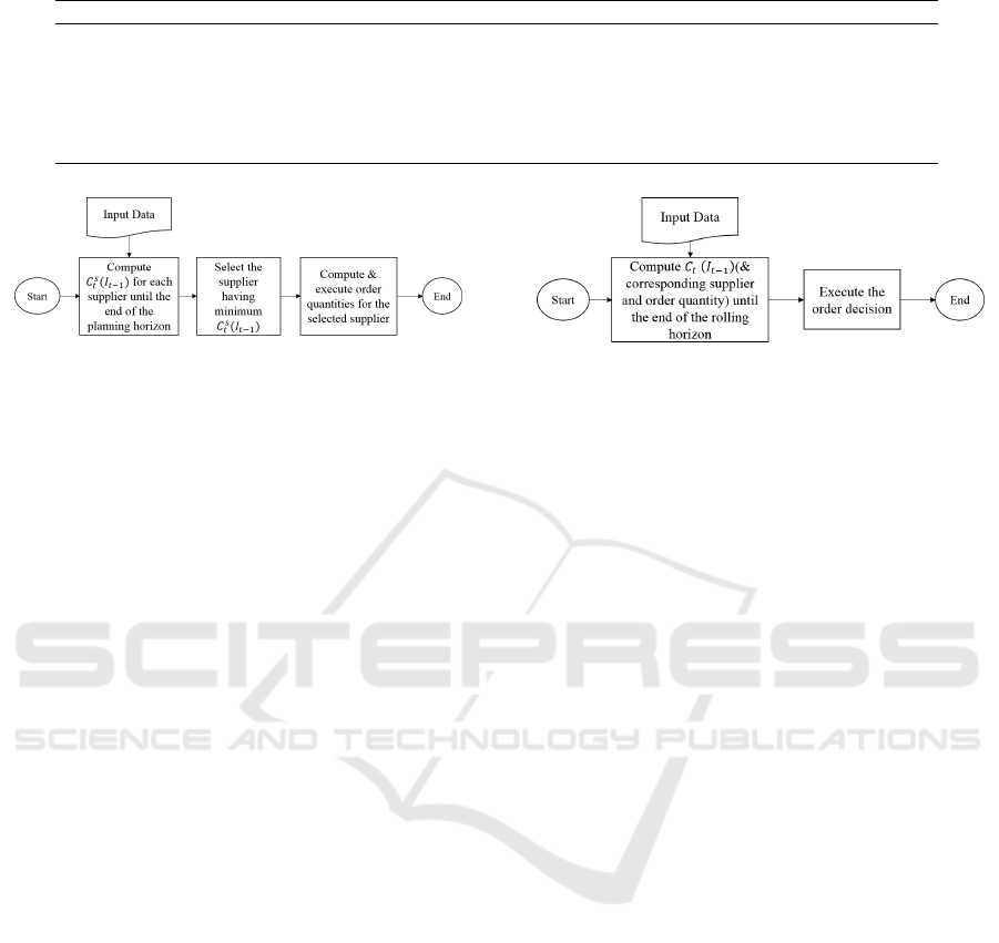
Table 2: MCPC Calculations.

t = 1 t = 2 ... ... t = T − 1 t = T

∗

, q, 1, 1)

∗

(0, q, 2, 2) ... ...

∗

(0, q, T − 1, T − 1)

∗

(0, q, T, T )

∗

, q, 1, 2)

∗

(0, q, 2, 3) ... ...

∗

(0, q, T − 1, T )

... ... ... ...

∗

, q, 1, T − 1)

∗

(0, q, 2, T )

∗

, q, 1, T )

Figure 2: Working of common supplier selection.

t, and q

being the actions

t−1

) = min





H(I

t−1

+ q

− d

)

+W [−I

t−1

− q

+ d

]

+ K

∑

s=1

+ C

t+1

t−1

+ q

− d

)





(1)

(

1 if q

> 0

0 otherwise

(2)

The ﬁrst, second, third and fourth terms represent

the expected inventory holding costs, expected short-

age costs, ﬁxed order cost and purchase costs respec-

tively for period t. The last term represents the min-

imum expected cost for the next period. The above

equation can be solved optimally by value iteration

(Puterman, 2014). The methodology is summarized

in Figure 2.

3.3 Dynamic Supplier Selection

The dynamic supplier selection problem is quite

similar to the common supplier problem except, it

has several sets of possible actions. In the case of

common supplier selection, we considered the set

of possible actions q

for each supplier s separately.

However, in case of a dynamic supplier selection, we

consider all possible actions from all possible sup-

pliers in a single dynamic program. The functional

equation is given below. With C

t−1

) being the

optimal cost with state I

t−1

at time t, and q

being

the actions

Figure 3: Working of dynamic supplier selection.

t−1

) = min

,s∈S





H(I

t−1

∑

s=1

− d

)

+W [−I

t−1

−

∑

s=1

+ d

]

∑

s=1

∑

s=1

+ C

t+1

t−1

∑

s=1

− d

)





(3)

In the above program, we do not consider the ca-

pacity constraint for the suppliers. Inclusion of capac-

ity constraint can affect the ordering decisions and,

we plan to study this in future research. Dynamic sup-

plier selection can be achieved using the above formu-

lation. Choice of supplier at an ordering epoch is af-

fected by the inventory position, unit purchase price,

ﬁxed order cost and minimum order quantities, etc.

The methodology is summarized in Figure 3.

3.3.1 Approximation Framework

The dynamic programs presented previously can be-

come intractable when the number of periods is high.

In this section we present an approximation frame-

work to alleviate the curse of dimensionality without

compromising the solution quality substantially.

We introduce a term called minimum coverage pe-

riod cost (MCPC) which is formally deﬁned as fol-

lows. Under the assumption of discrete time periods

the MCPC is the minimum expected cost during a

coverage period of length not less than one. A cov-

erage period is such that any order received in the

beginning would sufﬁce till the end. Our proposed

method has two major stages. The ﬁrst stage is a gen-

eral black box which gives the optimal order quantity

and cost for any discrete coverage period. Such meth-

ods are given in (Sahu et al., 2019) for any general

An Approximate Method for Integrated Stochastic Replenishment Planning with Supplier Selection

distributions and (

Ozen et al., 2012) for parametric

distributions. Once we get those costs, we can pro-

ceed to minimize the cost for the whole rolling hori-

zon in the second stage using a dynamic programming

approach XDP. The process is depicted in Figure 4.

Inputs

BLACK BOX XDP

Outputs

Figure 4: Illustration of the approximation framework. The

inputs required are current inventory level, demand infor-

mation and cost parameters. The BLACK BOX gives the

MCPC for any given coverage period. The XDP used those

costs to minimize the rolling horizon cost using a dynamic

program.

3.3.2 Rolling Horizon Cost Optimization

We propose a dynamic programming approach to

minimize the total cost over the rolling horizon. The

process is presented in Figure 5.

Let us consider a rolling horizon of length T . An

order can be placed at any time t ∈ {1, 2, ..., T }. When

the decision is taken at time t = 1, order can be placed

at any one of the suppliers s ∈ {1, 2, ..., S}. The order

quantity for any supplier can have coverage period

upto {1, 2, ..., T }. If we go further in time at t = 2,

we can have different ordering options based on the

state of inventory. However, our initial deﬁnition of

coverage period states that the delivered quantity suf-

ﬁces till the end of that coverage period. Therefore,

for each time period t > 1, we compute the optimal

order quantity and cost assuming the inventory state

equal to zero. Hence, if an ordering decision is made

at time t = 2 of the same rolling horizon, the order

quantity for any supplier can have coverage period

up to {2, 3, ..., T }. Similarly, if a ordering decision

is made at time t of the same rolling horizon, the

order quantity for any supplier can have coverage

period {t, t + 1, ..., T }. From the above we have, at

t = 1, there are ST ordering options, at t = 2, there

are S(T − 1) ordering options and so on. At t = T ,

there are S ordering options. Additionally, no order

option can also be adopted. Let

∗

, q, T

, T

)

represent the MCPC for supplier s, for the coverage

period T

to T

≥ T

). From the analysis given

in the paragraph above, all possible ordering options

during a rolling horizon of length T are given in

Table 2. Those values are provided by the BLACK

BOX along with corresponding order quantities.

Mathematically,

∗

, q, T

, T

) is deﬁned as fol-

lows.

∗

, q, T

, T

) = min E

∑

t=T



H[I

+ q

−

∑

τ=T

]

+W [−I

− q

∑

τ=T

]

+ R

+ α



(4)

The possible different

∗

, q, T

, T

) are presented

in Table 2. We end up with

T (T+1)

different costs for

a rolling horizon of length T . After the computation

of all the minimum expected costs, we can solve the

multi-stage problem for the whole rolling horizon us-

ing a dynamic programming formulation as presented

below. All the MCPCs are computed at zero initial

inventory.

= min

∗

(0, q, T, T ) (5)

T −1

= min



min



∗

(0, q, T − 1, T − 1) + Z



min



∗

(0, q, T − 1, T )



(6)

T −2

= min



min



∗

(0, q, T − 2, T − 2) + Z

T −1



min



∗

(0, q, T − 2, T − 1) + Z



min



∗

(0, q, T − 2, T )



(7)

= min



min



∗

(0, q, 1, 1) +Z



min



∗

(0, q, 1, 2) +Z



, ...,

min



∗

(0, q, 1, T − 1) + Z



min



∗

(0, q, 1, T )



(8)

The above formulation is a backward recursion.

At t = T , we have the option of ordering only to cover

the period T . Therefore, its expected minimum cost

is the minimum of expected costs across the suppliers

with coverage period T . Similar computations for the

whole rolling horizon is of the order

ST (T+1)

ICORES 2020 - 9th International Conference on Operations Research and Enterprise Systems

t = 1

t =

= 0, q, T

, T

)

= 1 T

= 1

, q, 1, 1)

= 1 T

= 2

, q, 1, 2)

Figure 5: Illustration of an ordering mechanism and cost computation with a rolling horizon length T and planning horizon

length

T . During each time period t order quantities are determined considering the opening inventory level and demand over

a t to t + T window. The black box stage give the optimal cost for all possible coverage periods T

to T

4 NUMERICAL RESULTS

In this section, we present the experimental protocol

and the detailed numerical results. To test the per-

formance of our proposed method, we compare its

cost with the optimal cost obtained with dynamic pro-

gramming.

4.1 Experimental Protocol

In the previous section, we have explained our pro-

posed two-stage method. In the ﬁrst stage, we ap-

proximate the minimum expected costs for all pos-

sible coverage periods. We use these costs to formu-

late a dynamic programming approach to compute the

minimum cost over the whole rolling horizon.

Our test-bed is as follows. At the beginning of

time period t = 1, the demand forecasts upto period

T are available. The decision maker uses this demand

information, current inventory and cost parameters to

compute the order quantity and places the ordered for

the ﬁrst period. The problem instances are presented

in Table 3. In the beginning, we start with inventory

= 0 and zero backorder. Any order placed is deliv-

ered immediately. A random demand following the

same distribution as forecast is received and the corre-

sponding excess inventory or backorder levels are up-

dated. The period cost is computed as the sum of ﬁxed

order cost, inventory cost and backorder cost. The

process is repeated until period T with demand infor-

mation of period {2, 3, ..., T }, {3, 4, ..., T } and so on

upto {T }. The total cost is then computed as the sum

of all period costs. We ﬁrst obtain the optimal cost of

the above process using dynamic programming. We

conduct simulation to assess the expected cost with

our proposed method. Since our method uses sam-

ples, we conduct 10

such simulations to estimate the

expected cost of the planning horizon. We conduct

tests for stationary demand that follow poisson dis-

tribution, with means equal to 5 and a planning hori-

zon length of 20 periods. For the ﬁrst set, inventory

costs are H = {1, 0.5, 0.1}, the backorder cost W = 20

and for second set, the inventory cost is kept ﬁxed at

H = 1 and backorder costs are W = {30, 25, 15}. Our

An Approximate Method for Integrated Stochastic Replenishment Planning with Supplier Selection

Table 3: Problem instances.

H W K

MOQ

Set − 1

1 20 [20,20,20,20] [10,9,8,7] 0

1 20 [20,40,80,150] [10,10,10,10] 0

1 20 [20,40,80,150] [10,9,8,7] 0

1 20 [20,40,80,150] [10,8,7,5] 0

0.5 20 [20,20,20,20] [10,9,8,7] 0

0.5 20 [20,40,80,150] [10,10,10,10] 0

0.5 20 [20,40,80,150] [10,9,8,7] 0

0.5 20 [20,40,80,150] [10,8,7,5] 0

0.1 20 [20,20,20,20] [10,9,8,7] 0

0.1 20 [20,40,80,150] [10,10,10,10] 0

0.1 20 [20,40,80,150] [10,9,8,7] 0

0.1 20 [20,40,80,150] [10,8,7,5] 0

Set − 2

1 30 [20,20,20,20] [10,9,8,7] 0

1 30 [20,20,40,80] [10,10,10,10] 0

1 30 [20,20,40,80] [10,9,8,7] 0

1 30 [20,20,40,80] [10,8,7,5] 0

1 25 [20,20,20,20] [10,9,8,7] 0

1 25 [20,20,40,80] [10,10,10,10] 0

1 25 [20,20,40,80] [10,9,8,7] 0

1 25 [20,20,40,80] [10,8,7,5] 0

1 15 [20,20,20,20] [10,9,8,7] 0

1 15 [20,20,40,80] [10,10,10,10] 0

1 15 [20,20,40,80] [10,9,8,7] 0

1 15 [20,20,40,80] [10,8,7,5] 0

Set − 3

1 20 [40, 40, 40, 40] [10, 9, 8, 7] [0,5,10,15]

1 20 [40, 40, 40, 40] [10, 9, 8, 7] [1,6,12,18]

1 20 [40, 40, 40, 40] [10, 9, 8, 7] [2,7,14,21]

1 20 [40, 40, 40, 40] [10, 9, 8, 7] [3,8,16,24]

1 20 [40, 40, 40, 40] [10, 9, 8, 7] [4,9,18,27]

1 20 [40, 40, 40, 40] [10, 9, 8, 7] [5,10,20,30]

1 20 [40, 40, 40, 40] [10, 9, 8, 7] [6,11,22,33]

1 20 [40, 40, 40, 40] [10, 9, 8, 7] [7,12,24,36]

1 20 [40, 40, 40, 40] [10, 9, 8, 7] [8,13,26,39]

1 20 [40, 40, 40, 40] [10, 9, 8, 7] [9,14,28,42]

1 20 [40, 40, 40, 40] [10, 9, 8, 7] [10,15,30,45]

1 20 [40, 40, 40, 40] [10, 9, 8, 7] [11,16,32,48]

Table 4: Comparison of optimal expected costs of common

supplier selection (CS) and dynamic supplier selection (DS)

approaches for input data Set − 1. Backorder cost W = 20,

MOQ = None.

H K

CS DS(Gain %)

1 [20,20,20,20] [10,9,8,7] 1032.0 1032.0(0.0)

1 [20,40,80,150] [10,10,10,10] 1331.8 1331.8(0.0)

1 [20,40,80,150] [10,9,8,7] 1331.8 1330.6(0.1)

1 [20,40,80,150] [10,8,7,5] 1245.3 1242.9(0.2)

0.5 [20,20,20,20] [10,9,8,7] 943.5 943.5(0.0)

0.5 [20,40,80,150] [10,10,10,10] 1244.4 1244.4(0.0)

0.5 [20,40,80,150] [10,9,8,7] 1230.2 1223.2(0.6)

0.5 [20,40,80,150] [10,8,7,5] 1107.4 1090.4(1.5)

0.1 [20,20,20,20] [10,9,8,7] 827.5 827.5(0.0)

0.1 [20,40,80,150] [10,10,10,10] 1130.1 1130.1(0.0)

0.1 [20,40,80,150] [10,9,8,7] 1032.0 1003.5(2.8)

0.1 [20,40,80,150] [10,8,7,5] 825.7 806.0(2.4)

problem has 4 suppliers. Their unit price, ﬁxed or-

der costs are presented in respective result tables. We

also test when minimum order quantity constraint is

also present. The rolling horizon length is set at 20

periods.

Table 5: Comparison of optimal expected costs of common

supplier selection (CS) and dynamic supplier selection (DS)

approaches for input data Set − 2. Inventory holding cost

H = 1, MOQ = None.

W K

CS DS(Gain %)

30 [20,20,20,20] [10,9,8,7] 1049.7 1049.7(0.00)

30 [20,40,80,150] [10,10,10,10] 1352.9 1352.9(0.00)

30 [20,40,80,150] [10,9,8,7] 1352.9 1350.7(0.17)

30 [20,40,80,150] [10,8,7,5] 1265.7 1262.7(0.24)

25 [20,20,20,20] [10,9,8,7] 1041.5 1041.5(0.00)

25 [20,40,80,150] [10,10,10,10] 1343.1 1343.1(0.00)

25 [20,40,80,150] [10,9,8,7] 1343.1 1341.3(0.13)

25 [20,40,80,150] [10,8,7,5] 1257.6 1254.5(0.24)

15 [20,20,20,20] [10,9,8,7] 1018.2 1018.2(0.00)

15 [20,40,80,150] [10,10,10,10] 1314.7 1314.7(0.00)

15 [20,40,80,150] [10,9,8,7] 1314.7 1313.4(0.10)

15 [20,40,80,150] [10,8,7,5] 1228.9 1227.2(0.14)

Table 6: Comparison of optimal expected costs of com-

mon supplier selection (CS) and dynamic supplier selection

(DS) approaches for input data Set − 3. Inventory hold-

ing cost H = 1, backorder cost W = 20, ﬁxed order costs

= [40, 40, 40, 40], Purchase prices R

= [10, 9, 8, 7].

MOQ CS DS Gain (%)

[0, 5, 10, 15] 1152.09 1149.01 0.27

[1, 6, 12, 18] 1156.56 1150.89 0.49

[2, 7, 14, 21] 1163.27 1154.51 0.76

[3, 8, 16, 24] 1172.33 1159.80 1.08

[4, 9, 18, 27] 1194.99 1171.65 1.99

[5, 10, 20, 30] 1209.36 1183.54 2.18

[6, 11, 22, 33] 1222.40 1195.97 2.21

[7, 12, 24, 36] 1264.04 1215.25 4.01

[8, 13, 26, 39] 1288.67 1235.14 4.33

[9, 14, 28, 42] 1304.23 1253.52 4.05

[10, 15, 30, 45] 1310.69 1271.93 3.05

[11, 16, 32, 48] 1317.82 1289.63 2.19

4.2 Results and Discussion

The results are divided into two parts. Tables 4, 5 and

6 present the comparison between the common sup-

plier selection and dynamic supplier selection. When

the suppliers are equivalent in terms of ﬁxed cost or

unit purchase price, both approaches yield equal cost.

Only when suppliers are different in both parameters,

there is a cost difference. The results from Tables 4,

5 show that the cost difference is higher when the

ratio of backorder cost to inventory holding cost is

higher. When the minimum order quantity constraint

is present, even with equal ﬁxed cost for all suppli-

ers, results show a cost different between both ap-

proaches. In each instance, dynamic supplier selec-

tion outperforms common supplier selection. The av-

erage runtime for common supplier selection is 2821

seconds on average.

In the second part, we present the results using our

proposed approximate method in Tables 7, 8 and 9

for the same problem instances. We get major gain in

terms of runtime. The average runtime of our method

is 6 milliseconds. The average error for the problem

ICORES 2020 - 9th International Conference on Operations Research and Enterprise Systems

Table 7: Comparison of approximate expected costs using XDP for common supplier selection (CS) and dynamic supplier

selection (DS) approaches for input data Set − 1. Inventory holding cost W = 20, MOQ = None.

H W K

CS Error(%) DS Error (%)

1 20 [20,20,20,20] [10,9,8,7] 1033.40 0.14 1033.40 0.14

1 20 [20,40,80,150] [10,10,10,10] 1347.88 1.20 1347.88 1.20

1 20 [20,40,80,150] [10,9,8,7] 1335.87 0.30 1332.54 0.14

1 20 [20,40,80,150] [10,8,7,5] 1246.06 0.06 1245.53 0.21

0.5 20 [20,20,20,20] [10,9,8,7] 948.54 0.53 948.54 0.53

0.5 20 [20,40,80,150] [10,10,10,10] 1260.60 1.30 1260.60 1.30

0.5 20 [20,40,80,150] [10,9,8,7] 1232.75 0.20 1226.30 0.26

0.5 20 [20,40,80,150] [10,8,7,5] 1117.98 0.95 1108.49 1.66

0.1 20 [20,20,20,20] [10,9,8,7] 836.30 1.07 836.30 1.07

0.1 20 [20,40,80,150] [10,10,10,10] 1133.79 0.32 1133.79 0.32

0.1 20 [20,40,80,150] [10,9,8,7] 1041.51 0.92 1010.19 0.67

0.1 20 [20,40,80,150] [10,8,7,5] 830.07 0.53 811.55 0.69

Average 0.63 0.68

Table 8: Comparison of approximate expected costs using XDP for common supplier selection (CS) and dynamic supplier

selection (DS) approaches for input data Set − 2. Backorder cost H = 1, MOQ = None.

H W K

CS Error(%) DS Error (%)

1 30 [20,20,20,20] [10,9,8,7] 1 059.74 0.96 1059.74 0.96

1 30 [20,20,40,80] [10,10,10,10] 1 383.74 2.28 1383.74 2.28

1 30 [20,20,40,80] [10,9,8,7] 1 381.00 2.07 1378.49 2.06

1 30 [20,20,40,80] [10,8,7,5] 1 266.37 0.05 1263.33 0.05

1 25 [20,20,20,20] [10,9,8,7] 1 051.27 0.93 1051.27 0.93

1 25 [20,20,40,80] [10,10,10,10] 1 353.66 0.79 1353.66 0.79

1 25 [20,20,40,80] [10,9,8,7] 1 383.64 3.02 1365.56 1.81

1 25 [20,20,40,80] [10,8,7,5] 1 261.35 0.30 1259.22 0.37

1 15 [20,20,20,20] [10,9,8,7] 1 030.42 1.20 1030.42 1.20

1 15 [20,20,40,80] [10,10,10,10] 1 369.00 4.13 1369.00 4.13

1 15 [20,20,40,80] [10,9,8,7] 1 349.40 2.64 1319.11 0.44

1 15 [20,20,40,80] [10,8,7,5] 1 235.79 0.56 1229.82 0.21

Average 1.58 1.26

Table 9: Comparison of approximate expected costs using XDP for common supplier selection (CS) and dynamic supplier

selection (DS) approaches for input data Set − 3. Inventory holding cost H = 1, backorder cost W = 20, ﬁxed order costs

= [40, 40, 40, 40], Purchase prices R

= [10, 9, 8, 7].

H W K

MOQ CS Error(%) DS Error (%)

1 20 [40, 40, 40, 40] [10, 9, 8, 7] [0,5,10,15] 1192.09 3.47 1178.31 2.55

1 20 [40, 40, 40, 40] [10, 9, 8, 7] [1,6,12,18] 1168.56 1.04 1154.84 0.34

1 20 [40, 40, 40, 40] [10, 9, 8, 7] [2,7,14,21] 1174.27 0.95 1172.75 1.58

1 20 [40, 40, 40, 40] [10, 9, 8, 7] [3,8,16,24] 1212.33 3.41 1162.70 0.25

1 20 [40, 40, 40, 40] [10, 9, 8, 7] [4,9,18,27] 1203.99 0.75 1187.47 1.35

1 20 [40, 40, 40, 40] [10, 9, 8, 7] [5,10,20,30] 1226.36 1.41 1217.51 2.87

1 20 [40, 40, 40, 40] [10, 9, 8, 7] [6,11,22,33] 1238.40 1.31 1214.87 1.58

1 20 [40, 40, 40, 40] [10, 9, 8, 7] [7,12,24,36] 1272.04 0.63 1224.24 0.74

1 20 [40, 40, 40, 40] [10, 9, 8, 7] [8,13,26,39] 1306.67 1.40 1259.84 2.00

1 20 [40, 40, 40, 40] [10, 9, 8, 7] [9,14,28,42] 1320.23 1.23 1270.82 1.38

1 20 [40, 40, 40, 40] [10, 9, 8, 7] [10,15,30,45] 1327.69 1.30 1274.98 0.24

1 20 [40, 40, 40, 40] [10, 9, 8, 7] [11,16,32,48] 1341.82 1.82 1317.23 2.14

Average 1.56 1.42

problem instance is less than 2% for both common

supplier selection and dynamic supplier selection

5 CONCLUSIONS

In this article, we address the integrated replenish-

ment planning and supplier selection problem. This

problem can be formulated as a multi-stage stochas-

An Approximate Method for Integrated Stochastic Replenishment Planning with Supplier Selection

tic problem. Due to the curse of dimensionality,

it is intractable for medium to large size problems.

For its practical importance and complexity, it has

received considerable attention in the literature post

2003, however, mostly as a measure of risk mitiga-

tion. Nowadays, multi-brand retailers face the prob-

lem during their day to day operation. This gives rise

to the need of its study as a economic option and the

development of faster optimization method. We ﬁrst

conduct the ﬁnancial beneﬁt analysis of dynamic sup-

plier selection versus selecting a common supplier for

the planning horizon. Then we propose an approxi-

mation framework for the dynamic supplier selection

problem.

A common supplier for the whole planning hori-

zon is a practically more appealing feature. However,

the dynamic supplier selection results in higher eco-

nomic beneﬁts. Both of the aforementioned prob-

lems are multi-stage stochastic optimization prob-

lems. However, the latter one is relatively more com-

plex due to its increased number of possible actions.

Numerical analysis suggest that the dynamic supplier

supplier selection approach always outperforms the

approach with one common supplier, especially when

the inventory holding costs and the backorder costs

are very different, and when the suppliers impose a

minimum order quantity constraints. Finding the op-

timal solutions of any of the above approaches is time

consuming. Hence, we develop an approximation

framework based on dynamic programming.

The framework works in two stages. The ﬁrst

stage is a general black box which gives the opti-

mal order quantity and cost for discrete coverage pe-

riod. We then end up with

T (T+1)

different costs for

a rolling horizon of length T . Afterwards, a dynamic

programming approach optimizes the total cost for the

rolling horizon. We conduct numerical analysis to at-

test the performance of our proposed method. For the

synthetic instances the approach provides near opti-

mal solution at a fraction of the computation time.

On average the optimality gap is 1.18%. The average

computation time is 6 milliseconds.

Future research aspects are to test the method in

lost sale environments and when the suppliers give

quantity discounts which are some of the common

practices nowadays in retail. Also, deeper analysis

can be done to suggest when the economic beneﬁts of

a dynamic supplier selection problems outweighs the

practical beneﬁts of selecting a common supplier.

REFERENCES

Berling, P. and Mart

ınez-de Alb

eniz, V. (2015). Dynamic

speed optimization in supply chains with stochastic

demand. Transportation Science, 50(3):1114–1127.

Berling, P. and Mart

ınez-de Alb

eniz, V. (2016). A charac-

terization of optimal base-stock levels for a multistage

serial supply chain. Naval Research Logistics (NRL),

63(1):32–46.

Cheaitou, A. and Van Delft, C. (2013). Finite horizon

stochastic inventory problem with dual sourcing: Near

myopic and heuristics bounds. International Journal

of Production Economics, 143(2):371–378.

Defourny, B., Ernst, D., and Wehenkel, L. (2012). Multi-

stage stochastic programming: A scenario tree based

approach to planning under uncertainty. In Deci-

sion theory models for applications in artiﬁcial intel-

ligence: concepts and solutions, pages 97–143. IGI

Global.

Homem-de Mello, T. and Bayraksan, G. (2014). Monte

carlo sampling-based methods for stochastic opti-

mization. Surveys in Operations Research and Man-

agement Science, 19(1):56–85.

Ozen, U., Do

gru, M. K., and Tarim, S. A. (2012).

Static-dynamic uncertainty strategy for a single-

item stochastic inventory control problem. Omega,

40(3):348–357.

Puterman, M. L. (2014). Markov Decision Processes.: Dis-

crete Stochastic Dynamic Programming. John Wiley

& Sons.

Rahdar, M., Wang, L., and Hu, G. (2018). A tri-level op-

timization model for inventory control with uncertain

demand and lead time. International Journal of Pro-

duction Economics, 195:96–105.

Rossi, R., Kilic, O. A., and Tarim, S. A. (2015). Piece-

wise linear approximations for the static–dynamic un-

certainty strategy in stochastic lot-sizing. Omega,

50:126–140.

Sahu, R. K., Dhaenens, C., Veerapen, N., and Davy, M.

(2019). A sample-based optimization approach for the

stochastic replenishment planning. Submitted.

Scarf, H. (1959). The optimality of (s, S) policies in the dy-

namic inventory problem. Technical report, Stanford

Univ Calif Applied Mathematics and Statistics Labs.

Yao, M. and Minner, S. (2017). Review of multi-supplier

inventory models in supply chain management: An

update. Available at SSRN 2995134.

ICORES 2020 - 9th International Conference on Operations Research and Enterprise Systems