Matching-aware Shape Simpliﬁcation

Enrico S. Miranda

1 a

, Rog

erio Lu

ıs C. Costa

1 b

, Paulo Dias

2 c

and Jos

e Moreira

2 d

IEETA, University of Aveiro, Portugal

DETI - IEETA, University of Aveiro, Portugal

Keywords:

Polygon Simpliﬁcation, Spatio-temporal Data, Shape Matching.

Abstract:

Current research has shown signiﬁcant interest in spatio-temporal data. The acquisition of spatio-temporal

data usually begins with the segmentation of the objects of interest from raw data, which are then simpliﬁed

and represented as polygons (contours). However, the simpliﬁcation is usually performed individually, i.e.,

one polygon at a time, without considering additional information that can be inferred by looking at the

correspondences between the polygons obtained from consecutive snapshots. This can reduce the quality

of polygon matching, as the simpliﬁcation algorithm may choose to remove vertices that would be relevant

for the matching and maintain other less relevant ones. This causes undesired situations like unmatched

vertices and multiple matched vertices. This paper presents a new methodology for polygon simpliﬁcation that

operates on pairs of shapes. The aim is to reduce the occurrence of unmatched and multiple matched vertices,

while maintaining relevant vertices for image representation. We evaluated our method on synthetic and real

world data and performed an extensive comparative study with two well-known simpliﬁcation algorithms.

The results show that our method outperforms current simpliﬁcation algorithms, as it reduces the amount of

unmatched vertexes and of vertexes with multiple matches.

1 INTRODUCTION

Over the last few decades, the amount of geograph-

ical data being generated is increasing greatly. De-

velopments in sensor technology have expanded the

availability of geographical data being used for sev-

eral purposes. With the growing body of spatial data,

there is also an increasing demand for tools to deal

with spatio-temporal data. The applications can be as

diverse as monitoring Glacier-Ocean boundaries, for-

est cover and iceberg tracking.

Spatio-temporal data is often acquired at discrete

times and represented as an ordered sequence of snap-

shots. Each snapshot consists of a timestamp and a

geometry. The acquisition of each snapshot can be

summarized in the following steps: 1) obtain the raw

data, 2) use image segmentation to extract the con-

tour of the objects of interest and 3) apply simpliﬁca-

tion of the contour to obtain the polygon to be stored

in a database. These steps are depicted in Figure 1.

The extracted polygons are then interpolated as slices

https://orcid.org/0000-0003-1483-8448

https://orcid.org/0000-0003-2306-7585

https://orcid.org/0000-0002-3754-2749

https://orcid.org/0000-0003-4633-6944

between two shapes (McKenney and Webb, 2010).

Thus, spatio-temporal data can be represented by a

geometry and a function used to represent its evolu-

tion over time (Forlizzi et al., 2000). Such high-level

abstraction model treats real world entities as moving

points, moving lines or moving regions. One key as-

pect of such representation is the selection of the func-

tion used to represent the data evolution, which is of-

ten called in the context of moving regions as Region

Interpolation Problem (Tøssebro and G

uting, 2001;

Heinz and G

uting, 2016). The interpolation methods

derive the function of transition for a pair of shapes,

and build the whole evolution by interpolating each

pair of shapes sequentially. Any simpliﬁcation algo-

rithm that can be applied to a pair shapes can be used

on the snapshots being interpolated. It can then be ap-

plied to a whole time series, two snapshots at a time,

on the same way that interpolation methods are exe-

cuted.

Region interpolation methods often require the

deﬁnition of a matching between the vertices of two

shapes representing an object of interest in two con-

secutive observations. Shape Matching or Vertex Cor-

respondence Problem is the process of ﬁnding good

matches (Liu et al., 2004; Van Kaick et al., 2011).

Miranda, E., Costa, R., Dias, P. and Moreira, J.

Matching-aware Shape Simpliﬁcation.

DOI: 10.5220/0008969402790286

In Proceedings of the 15th International Joint Conference on Computer Vision, Imaging and Computer Graphics Theory and Applications (VISIGRAPP 2020) - Volume 1: GRAPP, pages

279-286

ISBN: 978-989-758-402-2; ISSN: 2184-4321

279

(a) Raw data (b) Segmented

data

traction

(d) Simpliﬁed

Polygon

Figure 1: Data acquisition process.

There are two main issues that can arise during

shape matching. First, some vertices in a shape may

have no corresponding vertices in the other shape.

Second, two or more vertices in a shape may cor-

respond to a single vertex in the other shape. Such

problems may be inﬂuenced by the simpliﬁcation al-

gorithm. Since some interpolation methods require

an one-to-one correspondence between the vertices

of the two shapes (Moreira et al., 2016), a post-

processing step is usually need to ﬁx these issues.

This paper presents a novel technique for simpli-

ﬁcation with a focus on matching that we call Match-

ing Aware Simpliﬁcation (MAS). Our technique is

meant to be applied to two shapes of the same ob-

ject at different times or in shapes to be matched.

The focus is on preserving vertices that are impor-

tant to deﬁne a correspondence with vertices of the

other shape, which would be discarded by other

simpliﬁcations algorithms (e.g. Ramer-Douglar-

Peucker algorithms (Douglas and Peucker, 1973)

and Visvalingam-Whyatt algorithm (Visvalingam and

Whyatt, 1993)). Our technique is able to deliver poly-

gons that lead to better automatic vertex matching.

We evaluate the results on real world and artiﬁcial

data, and we perform a wide numeric evaluation over

a publicly available dataset.

This paper is organized as follows. The next sec-

tion presents an overview on related work. Section 3

details the proposed method. Section 4 presents the

experimental results. Finally, Section 5 presents the

conclusion and guidelines for future work.

2 BACKGROUND AND RELATED

WORK

2.1 Polygon Simpliﬁcation

Image segmentation algorithms return all pixels (ver-

tices) deﬁning the boundaries of an object of inter-

est. That means the representation of the objects’ ge-

ometry is noisy and may have hundreds or thousands

of vertices. However, a large number of vertices can

be detrimental to the performance of algorithms, e.g.,

to ﬁnd a correspondence between the vertices of two

shapes (Shape Matching), or to estimate the transfor-

mation of an object between two snapshots (Region

Interpolation). In addition, noisy boundaries can cre-

ate unwanted behavior during the interpolations.

Boundaries and shapes can be simpliﬁed using

different families of algorithms. The ﬁrst algorithm

for simpliﬁcation was the Ramer-Douglas-Peucker

(RDP) algorithm, published in 1972 (Ramer, 1972)

and 1973 (Douglas and Peucker, 1973). In the RDP

algorithm, a line segment is deﬁned between the ﬁrst

and last vertexes of a polyline to be simpliﬁed. Then,

the most distant vertex from this line segment is in-

cluded in the simpliﬁed line (a polyline) - as long as

the vertex distance is over an accepted threshold value

(ξ). This process is now applied recursively on all sub

lines on the polyline until there are no vertices over ξ

distance from the line. In order to apply this process

to a polygon, we need to pick two vertices as refer-

ence vertices for the polylines.

Another common approach to polygon simpliﬁ-

cation is using Visvalingam-Whyatt (VW) algorithm

(Visvalingam and Whyatt, 1993). In the VW algo-

rithm, for every vertex in a line or polygon, we build

a triangle between this vertex and the previous and

next vertices. Then, the area of each triangle is calcu-

lated, and all vertices of triangles with an area below

a threshold ξ are removed. This process is applied

iteratively until no triagle has an area below ξ.

Accounting that the morphing or interpolation

happens between two different shapes, one can use

this additional information to create different simpliﬁ-

cations. Baxter et al. (Baxter III et al., 2009) proposed

a method for compatible embedding of two shapes,

and later generalized the approach for multiple shapes

(Baxter et al., 2009). This method reduces the num-

ber of vertices on a polygon, however to keep the

textures inside the polygon during the morphing pro-

cess, the reduction of vertices aims at embedding and

not at simpliﬁcation of the geometry. While suited

for morphing animations, embedding creates defor-

mations on the polygon when used on real world data.

GRAPP 2020 - 15th International Conference on Computer Graphics Theory and Applications

280

Take iceberg tracking for instance, where one would

rather be close to the original shape and area than en-

sure embedding on a bigger polygon that loses infor-

mation.

These techniques are characteristic in that they are

suited for simpliﬁcation of a single polygon or poly-

line, with minimal information loss (RDP and VW),

or they are suited for animation (embedding). But

they have no regard to the temporal behaviors of the

shape. Our method, on the other hand, uses the infor-

mation of two consecutive representations of the same

shape in order to simplify each object. We maintain

vertices that are more relevant to represent the tempo-

ral evolution of the object.

2.2 Shape Matching

In order to use the region interpolation functions on

the continuous spatio-temporal data representation,

simpliﬁed polygons generated for consecutive snap-

shots need to be matched. The matching can be based

on segments or concavities (Tøssebro and G

uting,

2001) (McKenney and Webb, 2010) or based on ver-

tices (Moreira et al., 2016) (Baxter III et al., 2009).

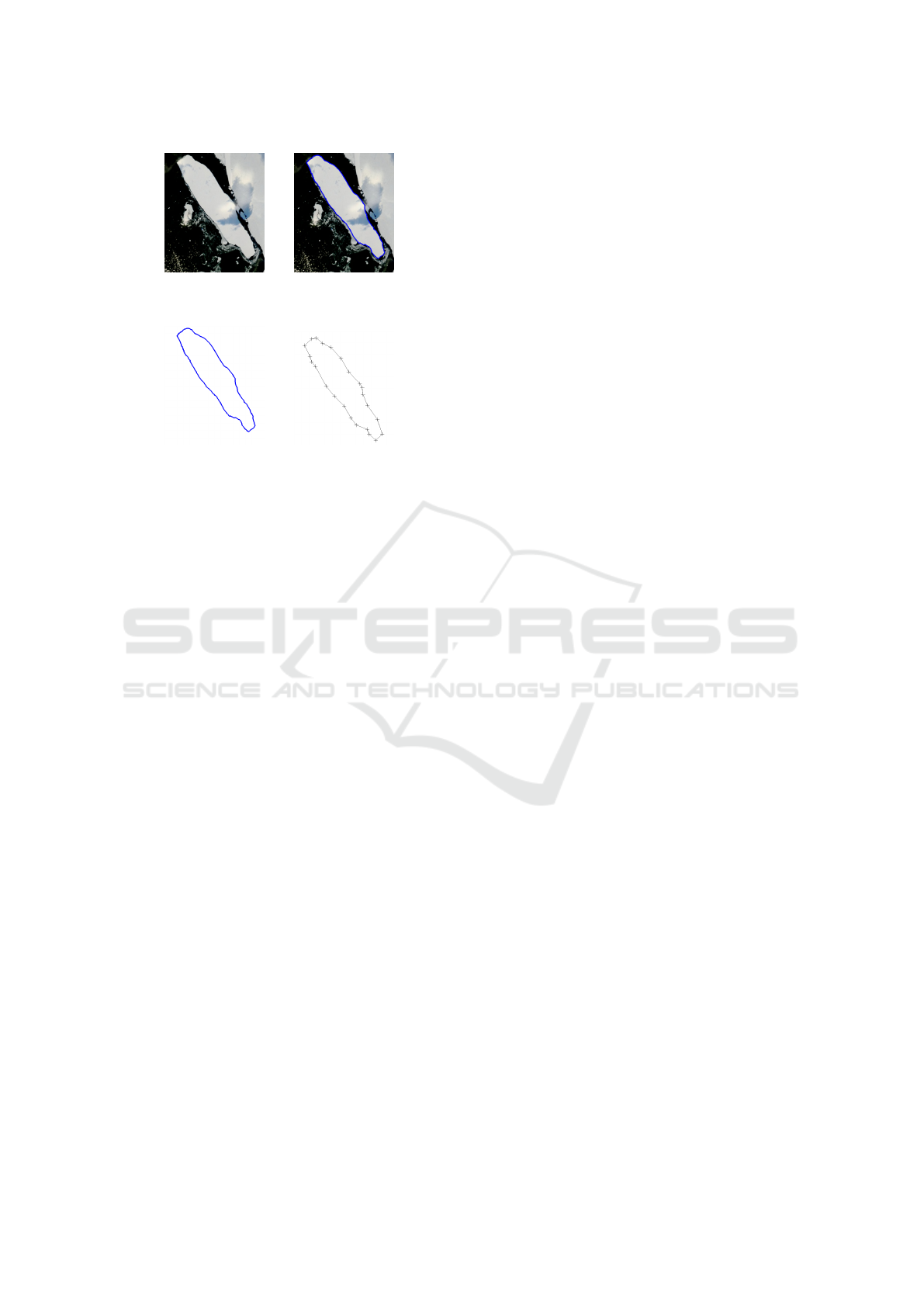
The Shape Matching algorithms must provide a cor-

respondence between the vertices of two shapes, as

depicted in Figure 2. It can also be seen that some

vertices might have no match, or match more than one

vertex. There are surveys on Shape Matching or Ver-

tex Correspondence Problem (Van Kaick et al., 2011).

Figure 2: Vertex matching (Van Kaick et al., 2007).

One algorithm with good results for fully auto-

matic 2D vertex matching is presented on (Van Kaick

et al., 2007). This algorithm performs vertex match-

ing so that the vertices matched are both in simi-

lar places in space, while also aiming at keeping the

geodesic distance (distances within the contour) be-

tween every pair of vertices similar. The additional

requirement that a pair of vertices in one shape main-

tain similar distances to the matched pair of vertices

on the other shape leads to a matching that is rela-

tively robust.

Since the existing simpliﬁcation algorithms are fo-

cused exclusively on the simpliﬁcation of shapes one-

by-one, two implications arise: 1) the simpliﬁcation

may select vertices in a shape that are distant from the

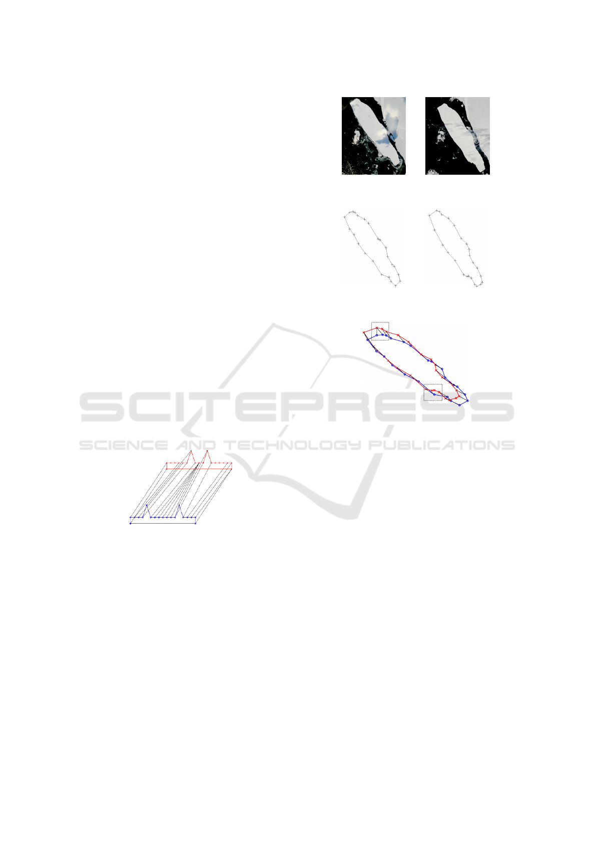
(a) Raw data from

ice01

(b) Raw data

from ice02

ice01

(d) Polygon from

ice02

(e) Vertex matching for B-15a

Figure 3: B-15a extraction and matching.

possible corresponding vertices in the other shape; or

2) the corresponding parts of two shapes may have

a different number of vertices. These cases are de-

picted in Figure 3, where the two polygons represent

the shape of iceberg B-15a at different times (from

now on called ice01 and ice02). The shapes were sim-

pliﬁed using RDP and the correspondences between

the vertices were performed using (Van Kaick et al.,

2007).

3 MULTIPLE-SHAPE AWARE

SIMPLIFICATION

The workﬂow to prepare spatio-temporal data

for interpolation can be summarized in 3 main

steps (Duarte et al., 2018). First, we extract the

region-of-interest from each raster image (Segmenta-

tion). Then, the amount of vertices on the shape is

reduced (Simpliﬁcation). Finally, a one-to-one corre-

spondence between the vertices must be found. In this

workﬂow, only the third step takes into account more

than one shape. We aim to improve this process by ex-

Matching-aware Shape Simpliﬁcation

281

tending the use of information from a pair of shapes

into the simpliﬁcation step, reducing matching errors.

3.1 Compatible Simpliﬁcation

Our method relies on implicit information, as we

know that we are simplifying a pair of related shapes

instead of an individual shape. We call this simpli-

ﬁcation of two shapes simultaneously as compatible

simpliﬁcation. The aim is to be able to consider the

importance of the vertices to represent a shape at a

given time and also their importance to establish cor-

respondence with vertices in the other shape. For in-

stance, we want to keep vertices that represent dis-

tinct features in a shape. We also want vertices that

should represent that distinct feature in the matched

shape. Our method operates before the vertex corre-

spondence problem, avoiding the need of optimiza-

tion and user interaction. This method can also be

paired with any correspondence algorithm.

Our method has two main objectives and one mi-

nor objective. The ﬁrst is to simplify a polygon in a

way that will reduce the need for adjustments during

the matching step, like adding extra vertices to solve

the vertex correspondence problem. Notice that the

added vertices were part of the full set of vertices be-

fore simpliﬁcation. Re-adding a vertex into a contour

that was removed during simpliﬁcation means that lo-

cal information was lost. Since our method deals with

simpliﬁcation using knowledge that is relevant to per-

form vertex correspondences in a later step, we are

call it Matching Aware Simpliﬁcation (MAS). Our

proposed method strives to keep vertices that will be

representative on future or past shapes by design.

The second main objective is to allow sim-

pler matching by providing matching algorithms

with locally-aware vertices in order to reduce ver-

tex matching complexity. Since algorithms can work

with locality of data in order to help ﬁnding the ver-

tex correspondences (Van Kaick et al., 2011), provid-

ing the algorithms with better locality should help the

matching process.

In order to keep vertices that allow better match-

ing, similar sub regions should be represented with

similar resolution or density of vertices. This minor

objective follows from the two main objectives.

3.2 The MAS Algorithm

In the following, we consider the raw contours to be

simpliﬁed as P, the source polygon, and the matched

polygon as Q, the target polygon. We assume that P

and Q were previously aligned to account for both ro-

tation and translation. We also deﬁne p ∈ P and q ∈ Q

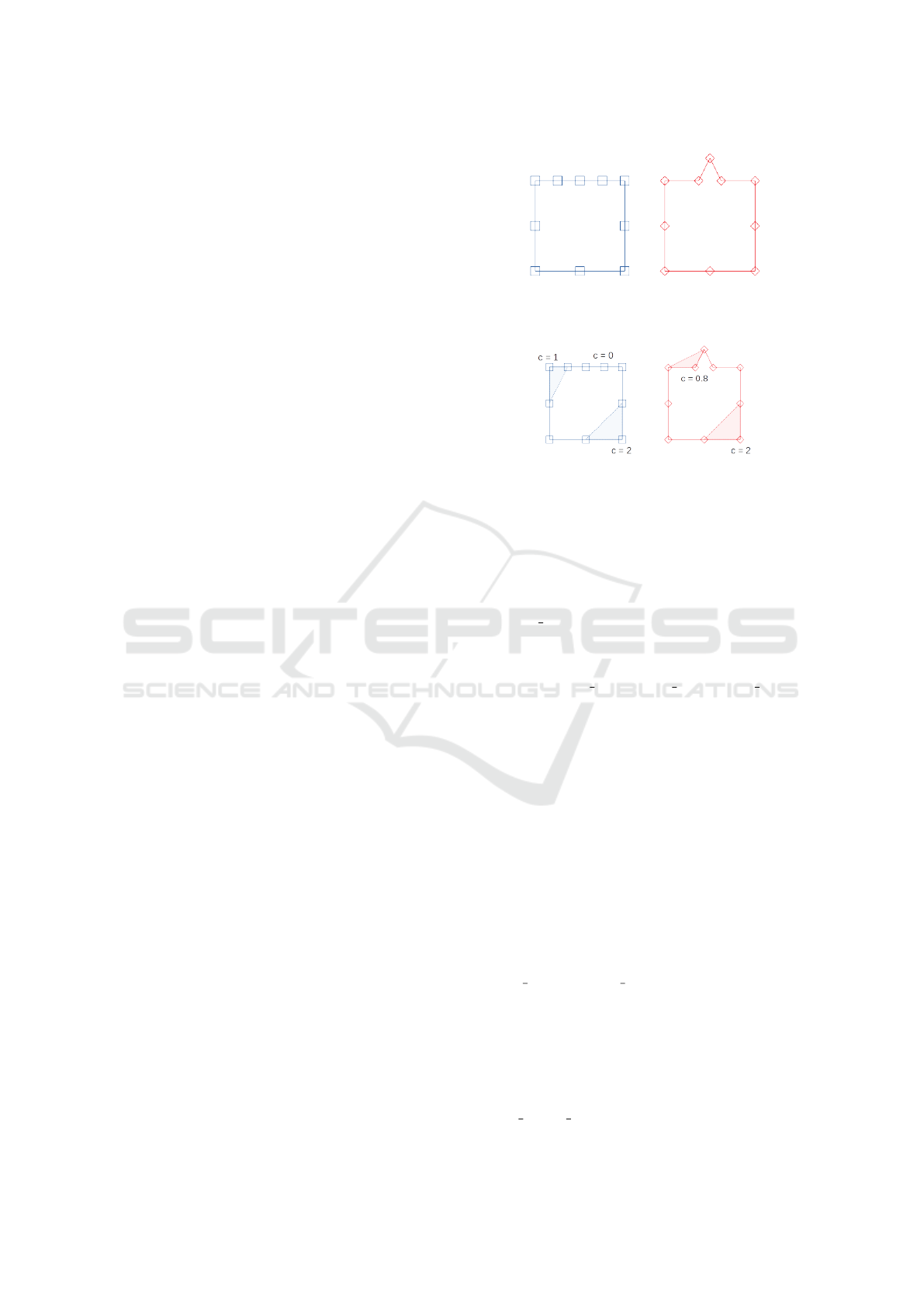
(a) Source (P) (b) Target (Q)

Figure 4: Artiﬁcial Polygons for illustration.

(a) Source (P) (b) Target (Q)

Figure 5: Local cost for vertices (triangle area).

as vertices. Figure 4 presents two artiﬁcial polygons

that will be used to illustrate cost calculations.

We start by deﬁning a cost function for each ver-

tex, which represents the loss of information for re-

moving this vertex (Equation 1). It introduces a pa-

rameter, t factor, representing the preference between

keeping temporal information or single shape infor-

mation.

cost

= max(cost single

, cost matched

∗t f actor)

(1)

In order to consider the loss of information on of

P and Q, we assume the cost to remove the vertex

p as the maximum of the cost to remove that vertex

considering a single shape (P) and of the cost for loss

of feature representation on the matched shape (Q).

We deﬁne the cost to remove a vertex for a single

shape as the area of the triangle given by p, p − 1 and

p + 1, similar to VW algorithm (Equation 2). It is

also possible to use other measures, like the distance

between p and the line connecting p − 1 and p + 1,

which would lead to a MAS simpliﬁcation based on

the RDP algorithm. Any future cost metric for single-

shape simpliﬁcation could also be applied at this step.

Figure 5 shows a calculation for some vertices.

cost single

= area triangle(p, p + 1, p −1) (2)

We represent the loss of matching information on

two different steps. A signiﬁcant vertex represents ei-

ther a feature present in Q and not in P, or a vertex

on P needed to morph into the feature of Q. The ﬁrst

case where P has a distinct and unique feature (like a

curvature or a distinctive deformation), the vertex has

a cost unique f eature as seen on Equation 3. This

GRAPP 2020 - 15th International Conference on Computer Graphics Theory and Applications

282

cost measures how distant the vertex is from the other

shape - a vertex far from the other shape represents a

distinct feature. Figure 6a shows this metric for three

different vertices of Q.

cost unique f eature

= min(d

)∀q ∈ Q)

(3)

(a) Distinct fea-

tures cost on Q (P

on background)

(b) Matching ver-

tices on P (Q on

background)

Figure 6: Matching costs.

We also deﬁne a cost for a matched feature, which

is complementary to the distinct feature. This cost is

deﬁned in Equation 4. This cost prioritizes vertices of

P that are the closest vertices for a distinct feature of

Q, and could be good candidates for future matching.

In the example in Figure 6b, the vertex at the top (with

c = 1) is important to morph into the topmost vertex

of Q.

cost matched f eature

= max(d

)∀q ∈ Q|

= min(d

)∀k ∈ P

(4)

Finally, we deﬁne the loss of information of vertex

p in the matching with Q as the maximum of the two

complementary costs, as seen on Equation 5.

cost time

= max(cost unique f eature

cost matched f eature

)

(5)

Given this deﬁnition of cost, our SIMPLIFY func-

tion starts by removing the vertex in P with lowest

cost, then removing the vertex in Q with lowest cost,

and iterating as many times as necessary to achieve

the desired number or vertices in the simpliﬁed poly-

gon.

function SIMPLIFY(P, Q, size)

while kPk > size ∨ kQk > size do

if kPk > size then

r ← p ∈ P|cost(p) = min(cost(k)∀k ∈

P ← P − r

end if

if kQk > size then

r ← q ∈ Q|cost(q) = min(cost(k)∀k ∈

Q ← Q − r

end if

end while

end function

4 EXPERIMENTAL RESULTS

In order to evaluate our proposals, we made several

experiments on publicly available datasets of artiﬁcial

and real world data, and compared the use of state-of-

the art simpliﬁcation algorithms. In all experiments,

the tolerance for each algorithm until 95% of the ver-

tices of the original contour were removed. This way,

the algorithms can be compared because they all keep

the same amount of information.

In Sections 4.1 and 4.2, we discuss the simpliﬁ-

cation quality presenting a visual analysis of selected

pairs of images. Then, in Section 4.3, we present a de-

tailed numeric comparison of MAS matching quality

(using several metrics) for every pair of image in the

216 Binary Shape Database from Brown University

(Sebastian et al., 2004).

4.1 Visual Qualitative Analysis -

Artiﬁcial Data

For the artiﬁcial data, we used two shapes from the

Brown University Binary Image dataset (Sebastian

et al., 2004), named arb01 and arb02. We can see

that for both arb01 and arb02 (Figure 7) the simpli-

ﬁed shapes cannot be visually distinguished from the

original image, leading to similar results of the con-

tour features.

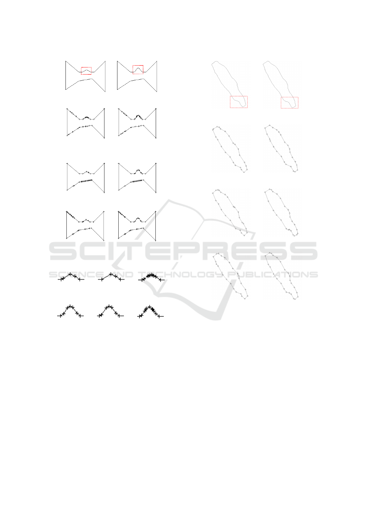
Considering arb01, the feature highlighted in Fig-

ure 8 can be represented using few vertices, since its

shape is triangular. However, in arb02, more vertices

are needed to represent the same feature, because the

shape is a round curve. It is important to keep a simi-

lar number of vertices in arb01 and arb02 for the ver-

tex matching. This is depicted in Figure 8, where the

simpliﬁcation algorithms are compared side-by-side,

showing how MAS keeps more points on the details

than both RDP and VW.

Our method chooses the vertices to be kept con-

sidering the context of the target shape. We can see

on Figure 7 that RDP and VW keep vertices on lines

that could be considered not-important (because they

do not play an important role on the deﬁnition of the

source and target shapes or on the deﬁnition of the

correspondences between them), like the lower in-

clined line in RDP or the left upper line in VW.

4.2 Visual Qualitative Analysis -

Real-world Data

For the real world data, we used two images of

Iceberg B-15a taken at different times (Figure 3)

(RossSea subsets, 2016). Each simpliﬁcation method

produces a slightly different shape, as we can see in

Matching-aware Shape Simpliﬁcation

283

(a) arb01 (b) arb02

arb01

(d) MAS on

arb02

(e) DP on arb01 (f) DP on arb02

(g) VW on arb01 (h) VW on arb02

Figure 7: Comparison of arb01 and arb02.

(a) VW on

arb01

(b) DP on

arb01

(d) VW on

arb02

(e) DP on

arb02

(f) MAS on

arb02

Figure 8: Highlight on the feature-area representation to all

simpliﬁcation algorithms.

Figure 9. However, the results of the methods are vi-

sually very similar.

It is visually perceptible in the highlighted area of

Figure 9 that the distribution of the vertices in the sim-

pliﬁed shapes is more similar in our method (consid-

ering the number of vertices and the spacing between

them). This better distribution of number of vertices

and spacing can also be seen on the left side of the

shape. Thus, our method performed as expected, pro-

viding more similar distributions of vertices on both

shapes with noisy borders.

(a) ice01 (b) ice02

(e) DP on ice01 (f) DP on ice02

(g) VW on ice01 (h) VW on ice02

Figure 9: Comparison of ice01 and ice02.

When dealing with real world data the borders are

noisy, and the noise can inﬂuence RDP or VW on se-

lecting the vertices to keep. Our goal was to remove

these inﬂuences by using information from the other

polygon and we can see in Figure 9 that our method

provides a more similar density of vertices along the

boundaries.

4.3 Simpliﬁcation and Matching

Analysis - Binary Shape Database

In order to provide a complete evaluation, we applied

our method on the 216 Binary Shape Brown dataset

(Sebastian et al., 2004). It is composed of 216 images

divided in 18 classes. This dataset is widely used in

polygon matching and image retrieval benchmarks.

GRAPP 2020 - 15th International Conference on Computer Graphics Theory and Applications

284

For the testing, we ﬁrst aligned the shapes using

the Iterative Closest Point method (Tihonkih et al.,

2016). For the hammer class the ICP method failed

to provide several correct rotations of the objects, and

so, they were removed from the test dataset.

We evaluated the performance of the simpliﬁca-

tion in the Vertex Correspondence Problem. For

this test, we used the VCP algorithm developed by

(Van Kaick et al., 2007) and recorded the number of

vertices without a correspondence and the number of

vertices with multiple matches, and considered both

cases as anomalous vertices.

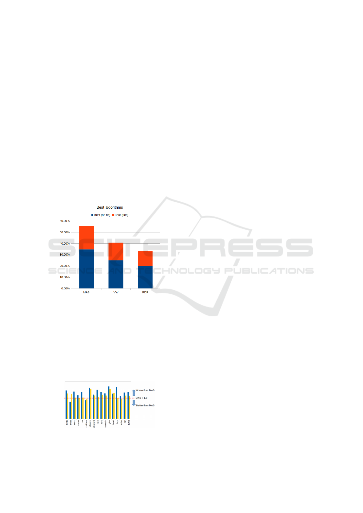
Since the VCP algorithm is an heuristic, it can

generate distinct results on consecutive executions.

To account for this, we ran 35 replications for each

pair of images. Our method was able to be the better

than RDP and VW on 35% of the images, and being

the best tied with either RDP or VW on 21%. Thus,

our method was the best choice on more than half of

the images. The results can be seen on Figure 10.

Figure 10: Performance comparison between algorithms.

It is also important to evaluate the gap of perfor-

mance instead of just which algorithm is best. For

this analysis, we compared the number of anomalous

points generated by each method. Figure 11 presents

these results. Our method is able to improve by a

wide margin on some categories. However, when our

method is not the best the gap is much smaller. Over-

all, our method can perform signiﬁcantly better on the

majority of the cases, or slightly worse on a few cases.

Figure 11: Anomalous vertices generated.

Finally, we selected a pair of shapes for visual as-

sessing of our method (Figure 12). It can be seen

that MAS represents all fork prongs with 2 points in

both shapes. Both VW and RDP chose to simplify

matching prongs with a different number of points

on each shape. Also, on the fork handle,the number

of pointed obtained using VW and RDP greatly dif-

fers, and MAS performs with closer density on both

shapes. These ﬁndings are highlighted in the images.

5 CONCLUSION

Current technology has enabled us to gather a rich set

of spatial data, leading to a growing body of historical

data. This has led to an increased interest in spatio-

temporal data processing and analysis.

Using the continuous spatio-temporal model to

represent real world data involves several steps, in-

cluding image acquisition and segmentation, object

simpliﬁcation and shape matching. Although data ac-

quisition can have a signiﬁcant impact on the quality

of the data, few works exist on transforming raw data

into spatio-temporal data representations. Also, after

image acquisition and segmentation the set of points

of the contour has to be simpliﬁed in order to obtain

a polygon. Current simpliﬁcation algorithms account

only for a single shape at a time. This can lead to a

loss of information about the evolution of the shapes

over time.

In this work, we deal with shape simpliﬁcation

for polygon matching. We presented an algorithm

for simpliﬁcation of 2D polygons. Our method

makes use of implicit information that arises from

the knowledge that we have more than one shape

to be matched. Our Matching Aware Simpliﬁca-

tion method improves simpliﬁcation quality, leading

to less anomalous points during matching than other

simpliﬁcation methods. Our method can also be com-

bined with any matching algorithm on the next stage

leading to improved matching results. The proposed

simpliﬁcation technique should allow for easier auto-

matic correspondence of vertices on real world phe-

nomena shapes.

In the future, we are interested in expanding re-

search on the next step of the spatio-temporal acqui-

sition workﬂow: the vertex correspondence problem.

Since it is expected that avoiding to remove vertices

from a shape (source) that may have a correspondence

with vertices of another shape (target) in a sequence of

observations will lead to more natural interpolations,

we also aim at developing workﬂows to evaluate the

impact of each step of the process on the quality of the

Matching-aware Shape Simpliﬁcation

285

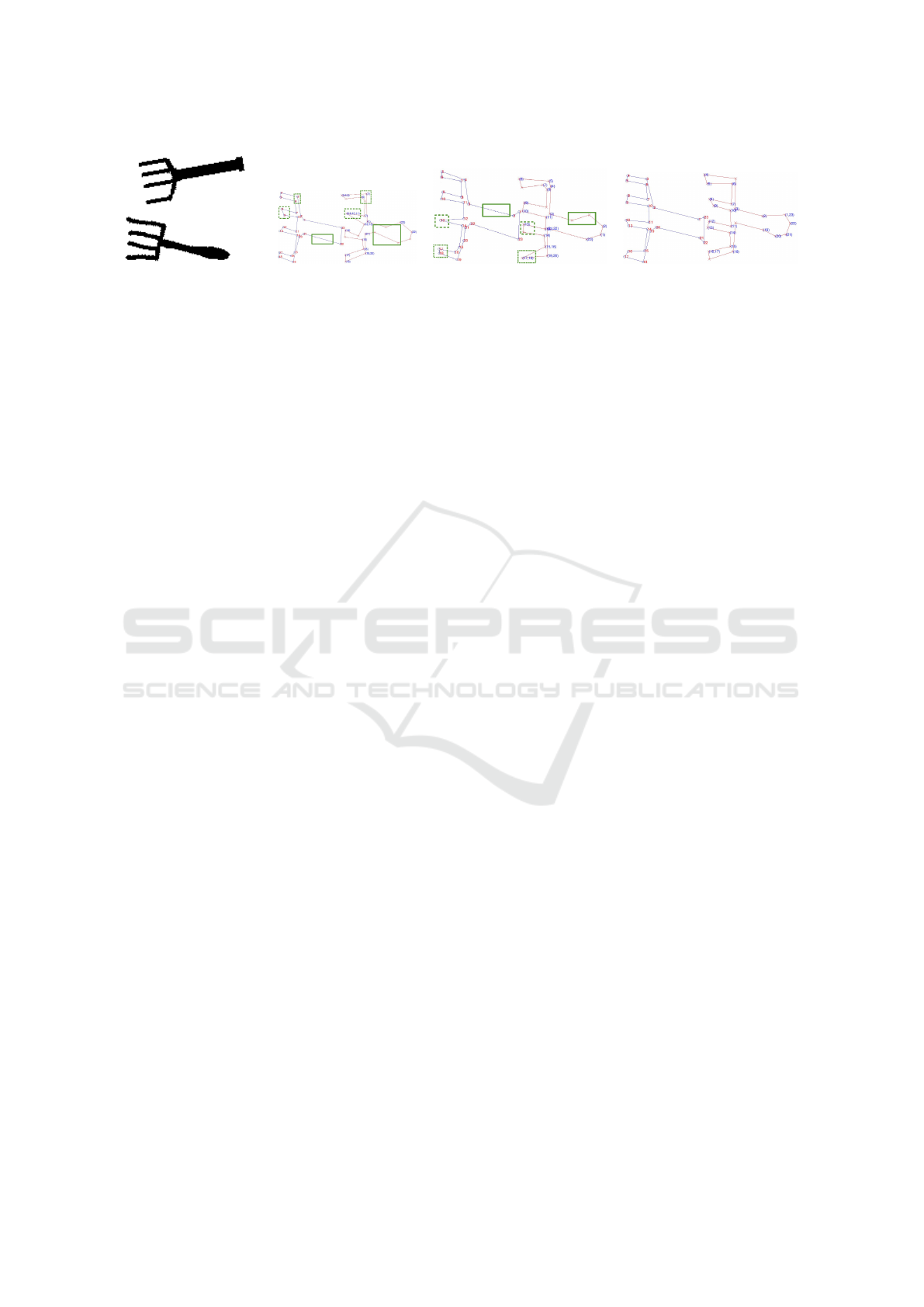
(a) Fork19.pgm and

Fork03.pgm

(b) VW matching (c) RDP matching (d) MAS matching

Figure 12: Matchings between Fork03 and Fork19.

interpolations. Finally, we would also want to work

on all steps of the interpolation process of multiple

snapshots, instead of two - including simpliﬁcation,

matching and interpolation functions.

ACKNOWLEDGEMENTS

This work is partially funded by National Funds

through the FCT in the context of the projects

UID/CEC/00127/2013 and POCI-01-0145-FEDER-

032636.

REFERENCES

Baxter, W., Barla, P., and Anjyo, K. (2009). N-way morph-

ing for 2d animation. Computer Animation and Vir-

tual Worlds, 20(2-3):79–87.

Baxter III, W. V., Barla, P., and Anjyo, K.-i. (2009). Com-

patible embedding for 2d shape animation. IEEE

Transactions on Visualization and Computer Graph-

ics, 15(5):867–879.

Douglas, D. H. and Peucker, T. K. (1973). Algorithms for

the reduction of the number of points required to rep-

resent a digitized line or its caricature. Cartographica:

the international journal for geographic information

and geovisualization, 10(2):112–122.

Duarte, J., Dias, P., and Moreira, J. (2018). An evaluation

of smoothing and remeshing techniques to represent

the evolution of real-world phenomena. In Interna-

tional Symposium on Visual Computing, pages 57–67.

Springer.

Forlizzi, L., G

uting, R. H., Nardelli, E., and Schneider, M.

(2000). A data model and data structures for moving

objects databases. In Proceedings of the 2000 ACM

SIGMOD International Conference on Management

of Data, SIGMOD ’00, pages 319–330, New York,

NY, USA. ACM.

Heinz, F. and G

uting, R. H. (2016). Robust high-quality

interpolation of regions to moving regions. GeoInfor-

matica, 20(3):385–413.

Liu, L., Wang, G., Zhang, B., Guo, B., and Shum, H.-Y.

(2004). Perceptually based approach for planar shape

morphing. In Proceedings of the Computer Graphics

and Applications, 12th Paciﬁc Conference, PG ’04,

pages 111–120, Washington, DC, USA. IEEE Com-

puter Society.

McKenney, M. and Webb, J. (2010). Extracting moving

regions from spatial data. In Proceedings of the 18th

SIGSPATIAL International Conference on Advances

in Geographic Information Systems, GIS ’10, pages

438–441, New York, NY, USA. ACM.

Moreira, J., Dias, P., and Amaral, P. (2016). Represen-

tation of continuously changing data over time and

space: Modeling the shape of spatiotemporal phenom-

ena. In 2016 IEEE 12th International Conference on

e-Science (e-Science), pages 111–119. IEEE.

Ramer, U. (1972). An iterative procedure for the polygonal

approximation of plane curves. Computer graphics

and image processing, 1(3):244–256.

RossSea subsets (2016). Rosssea subsets.

http://rapidﬁre.sci.gsfc.nasa.gov/imagery/ sub-

sets/?project=antarctica&subset=RossSea&

date=11/15/20. Accessed: 2016-09-20.

Sebastian, T. B., Klein, P. N., and Kimia, B. B. (2004).

Recognition of shapes by editing their shock graphs.

IEEE Transactions on Pattern Analysis & Machine In-

telligence, (5):550–571.

Tihonkih, D., Makovetskii, A., and Kuznetsov, V. (2016).

A modiﬁed iterative closest point algorithm for shape

registration. In Applications of Digital Image Process-

ing XXXIX, volume 9971, page 99712D. International

Society for Optics and Photonics.

Tøssebro, E. and G

uting, R. H. (2001). Creating represen-

tations for continuously moving regions from obser-

vations. In International Symposium on Spatial and

Temporal Databases, pages 321–344. Springer.

Van Kaick, O., Hamarneh, G., Zhang, H., and Wighton, P.

(2007). Contour correspondence via ant colony op-

timization. In 15th Paciﬁc Conference on Computer

Graphics and Applications (PG’07), pages 271–280.

IEEE.

Van Kaick, O., Zhang, H., Hamarneh, G., and Cohen-Or,

D. (2011). A survey on shape correspondence. In

Computer Graphics Forum, volume 30, pages 1681–

1707. Wiley Online Library.

Visvalingam, M. and Whyatt, J. D. (1993). Line general-

isation by repeated elimination of points. The carto-

graphic journal, 30(1):46–51.

GRAPP 2020 - 15th International Conference on Computer Graphics Theory and Applications

286