
Video Summarization through Total Variation, Deep Semi-supervised
Autoencoder and Clustering Algorithms
Eden Pereira da Silva
1
, Eliaquim Monteiro Ramos
1
, Leandro Tavares da Silva
1,2
, Jaime S. Cardoso
3
and Gilson A. Giraldi
1
1
National Laboratory for Scientific Computing, Petr
´
opolis, Brazil
2
Federal Center of Technology Education Celso Suckow da Fonseca, Petr
´
opolis, Brazil
3
INESC TEC and University of Porto, Porto, Portugal
Keywords:
Summarization, Cosine Similarity Metric, Total Variation, Autoencoder, K-means.
Abstract:
Video summarization is an important tool considering the amount of data to analyze. Techniques in this area
aim to yield synthetic and useful visual abstraction of the videos contents. Hence, in this paper we present a
new summarization algorithm, based on image features, which is composed by the following steps: (i) Query
video processing using cosine similarity metric and total variation smoothing to identify classes in the query
sequence; (ii) With this result, build a labeled training set of frames; (iii) Generate the unlabeled training set
composed by samples of the video database; (iv) Training a deep semi-supervised autoencoder; (v) Compute
the K-means for each video separately, in the encoder space, with the number of clusters set as a percentage of
the video size; (vi) Select key-frames in the K-means clusters to define the summaries. In this methodology,
the query video is used to incorporate prior knowledge in the whole process through the obtained labeled
data. The step (iii) aims to include unknown patterns useful for the summarization process. We evaluate the
methodology using some videos from OPV video database. We compare the performance of our algorithm
with the VSum. The results indicate that the pipeline was well succeed in the summarization presenting a
F-score value superior to VSum.
1 INTRODUCTION
Daily, millions of videos are posted online, and some
billions are available for public or private access,
as on YouTube, for example. This content is pro-
vided by professionals or amateurs recorders, with
many different devices as smartphones, surveillance
or traffic cameras, among others. If we can provide
some video summary, where the important informa-
tion along the video is captured, it will greatly reduce
the effort to browse through the enormous amount of
content available, during a content based video re-
trieval task. Video summarization can be described as
a subset selection problem, where the subsets contain
frames, sparsely distributed in the whole sequence,
or shots (set of temporally continuous interval-based
segments). In both cases, the subset is smaller than
the original video. The first case depends on key-
frames selection. The second case is implemented
through key shots selection.
In terms of pattern recognition tasks, two ap-
proaches are commonly applied to video summariza-
tion: unsupervised and supervised ones. The former
uses heuristics to satisfy some properties in order to
create summaries of the videos (Yuan et al., 2019; Li
et al., 2019). Supervised methods (Zhao et al., 2019;
Rochan et al., 2018) have access to raw videos and
their corresponding ground truth summaries. More-
over, they use mainly the advances on deep learn-
ing to construct summaries. Although the supervised
approaches have achieved better results than unsu-
pervised techniques, labeling data with the defined
ground-truth is not easily available.
A semi-supervised approach for fluid flow sum-
marization, in the context of computational fluid dy-
namics, is proposed in (Ramos et al., 2018), but the
authors did not present computational results. That
work suggests to use transferring learning (Hu et al.,
2016), combining labeled and unlabeled training sets
in order to allow an autoenconder (AE) to efficiently
learn how to encode samples in a reduced dimension
space. After the AE training, the data set is processed
by encoder and the feature vectors yielded enter into
a clustering algorithm for classification. In this paper,
Pereira da Silva, E., Ramos, E., Tavares da Silva, L., Cardoso, J. and Giraldi, G.
Video Summarization through Total Variation, Deep Semi-supervised Autoencoder and Clustering Algorithms.
DOI: 10.5220/0008969303150322
In Proceedings of the 15th International Joint Conference on Computer Vision, Imaging and Computer Graphics Theory and Applications (VISIGRAPP 2020) - Volume 4: VISAPP, pages
315-322
ISBN: 978-989-758-402-2; ISSN: 2184-4321
Copyright
c
2022 by SCITEPRESS – Science and Technology Publications, Lda. All rights reserved
315

we propose some improvements of this methodology
and its application in video summarization.
Specifically, the methodology proposed in
(Ramos et al., 2018) uses the following pipeline: (a)
build the labeled training set X
s
in the original space;
(b) perform a coarse temporal flow segmentation
using a simple similarity measure combined with an
interval tree analysis; (c) select key numerical frames
inside each obtained segment and assemble these
frames in a training set X
t
; (d) a semi-supervised AE
architecture is trained using the sets X
s
and X
t
to
generate a metric distance (encoding function); (e)
Apply X-means (Pelleg and Moore, 2000) clustering
technique, with the metric distance, to compute
the final partition of the frame sequence; (f) For
each obtained cluster, take a key-frame to build the
summarization sequence.
However, we have noticed that interval tree and
a simple distance metric (like Frobenius distance) do
not provide a satisfactory temporal segmentation in
the frames of videos. Futhermore, the X-means al-
gorithm tries to perform clustering without the need
to set a pre-defined number K of groups. However,
in the case of video sequences, the obtained results
are not satisfactory. Besides, it is not clear the ad-
vantages of a high cost semi-supervised AE against a
simpler unsupervised one. Therefore, in our work we
propose to use total variation denoising, followed by
differentiation and thresholding instead of the interval
tree. We also replace the distance metric by a similar-
ity measure based on the data correlation. Moreover,
we perform clustering using K-means instead of X-
means. We also compare a simple AE with the semi-
supervised AE proposed in (Ramos et al., 2018) to
evaluate the encoded quality of the former against the
latter. Up to the best of our knowledge, this is the
first work that applies a semi-supervised technique for
video summarization in a systematic procedure. The
whole methodology is the main contribution of this
paper.
The remaining text is organized as follows. Sec-
tion 2 we survey related works. In section 3 we
describe the background techniques. The proposed
methodology is presented in section 4. Next, section
5 discusses the computational experiments. Conclu-
sions and possible future works are presented in sec-
tion 6.
2 RELATED WORKS
A variety of video summarization techniques have
been proposed as seen in the literature (Yuan et al.,
2019; Zhao et al., 2019; Li et al., 2019; de Avila
et al., 2011). In this paper we focus only on the tech-
nique based on image features to construct the sum-
mary. Generally, those techniques can be classified
into unsupervised and supervised ones.
Clustering algorithms are one of the most popu-
lar unsupervised methodology. Given hand-craft fea-
tures, similar frames are grouped forming a cluster
and, from each cluster, the centers are taken to build
the summary. Also, some works in unsupervised class
use the frame histograms to learn clusters (de Avila
et al., 2011). In (Mohan and Nair, 2018) there is an
extension of this approach: the shot histograms are
compressed by a high-level feature extractor before
the clustering step. Other works construct models, as
in (Lei et al., 2019), where the video is modeled as
graph, where a graph vertex corresponds to a frame
and the edge between vertexes is weighted by the
Kullback-Leibler divergence of two frames based on
semantic probability distributions. A clustering and a
rank operation is applied on this graph method to cre-
ate the summary. Recent works in unsupervised sum-
marization have applied deep learning (Yuan et al.,
2019; Zhao et al., 2019; Jung et al., 2018), using in
general, convolutional or recurrent neural networks.
Deep learning is the principal tool in supervised
summarization approaches. In this case, the sum-
mary is modeled as a classification problem, where
in the ground truth, frames have labels that represent
classes in the video (Jung et al., 2018). However, even
with better results in video summarization, labeling
for many video frames is tedious task that depends on
the human intervention. Moreover, overfitting prob-
lems can frequently occur if no sufficient labeled data
is available. Therefore a semi-supervised approach,
which uses just one labeled video to summarize a set
of other videos, can mitigate these limitations being a
contribution to the area, which motivates our work.
3 TECHNICAL BACKGROUND
In mathematical terms, the total variation denoising
computes a smooth version of an input signal y ∈
R
N
by solving the optimization problem (Selesnick,
2012),
ˆx = arg min
x∈R
N
1
2
k
y − x
k
2
2
+ λkDxk, (1)
where x ∈ R
N
; λ is the smooth factor, and D is a ma-
trix (N − 1) × N described in (Selesnick, 2012).
An AE can be viewed as a special case of feed-
forward neural network that is trained to reproduce
its input at the output layer (Goodfellow et al., 2016).
The AE architecture is depicted in Figure 1. Both
VISAPP 2020 - 15th International Conference on Computer Vision Theory and Applications
316
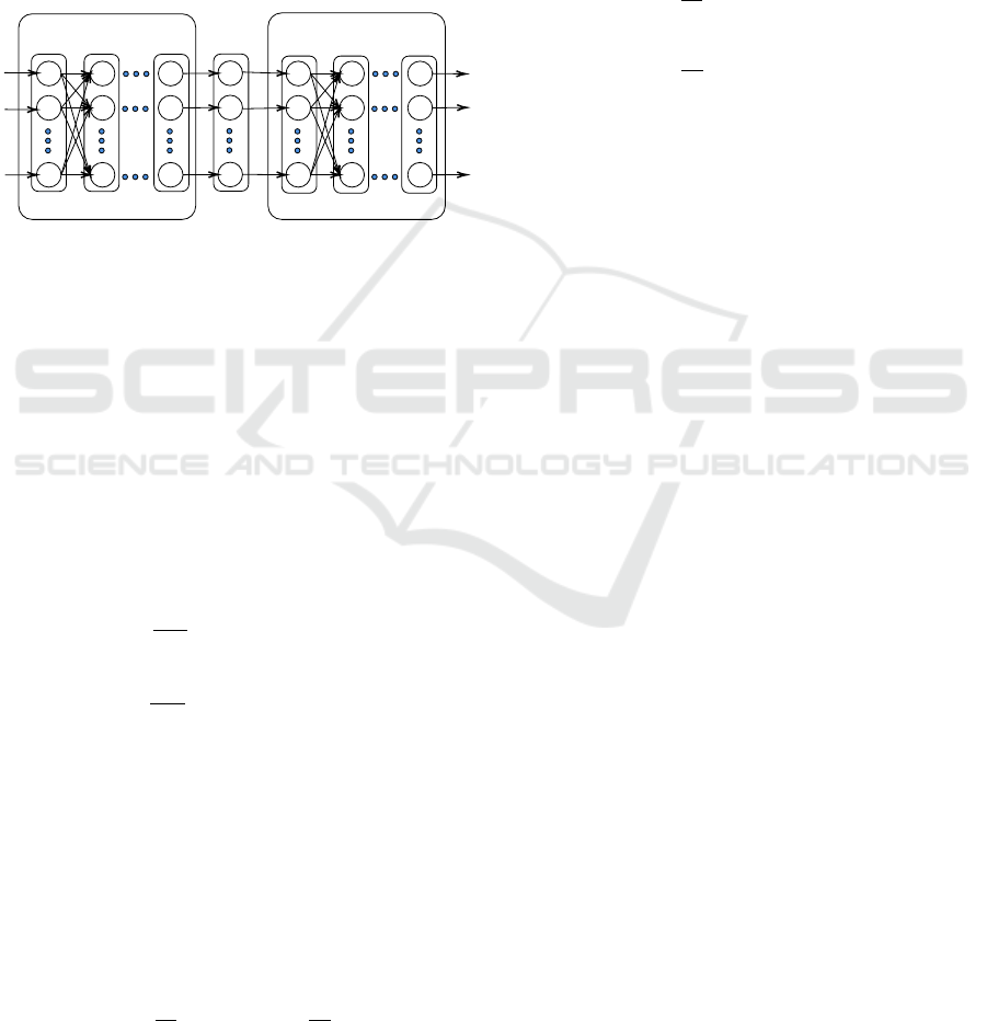
encoder and decoder in this figure are implemented
through a multilayer perceptron (MLP) neural net-
works where W
(ξ)
and b
(ξ)
are the weight matrix and
bias, respectively, for the layer ξ. Given an input V ,
the corresponding output V
(ξ)
at the ξ-th layer is com-
puted as:
f
(ξ)
(V ) = V
(ξ)
= ϕ
W
(ξ)
V
(ξ−1)
+ b
(ξ)
, (2)
where ϕ is a non-linear activation function (sigmoid
function, for instance), which operates component-
wisely.
f
(1)
f
(2)
f
(M)
f
(M+1)
f
(M+2)
f
(2M)
Encoder
Decoder
Coded
Input
V
(M)
W
(0)
b
(0)
W
(1)
b
(1)
W
(M)
b
(M)
W
(M+1)
b
(M+1)
W
(M+2)
b
(M+2)
W
(2M)
b
(2M)
Figure 1: Autoencoder (AE) graph representation. Com-
posed by one encoder and one decoder neural network. The
sets of weights on each AE layer are represented in matrix
form, where W
(m)
is the set of weights of the m-th layer.
On the same way, the bias for the m-th layer in represented
b
(m)
. Each f
(m)
represents the view of the layer as a trans-
formation. For an input x, f
(M)
(x), f
(2M)
(x) are the encoder
and decoder output respectively. The V
(M)
= f
(M)
(•) is the
output of the encoder.
The semi-supervised AE used in this work has
a loss function that incorporates the Fisher analysis,
based on the terms S
c
and S
b
, that represent the intra-
class variation and inter-class separation, respectively
(Hu et al., 2016):
S
(m)
c
=
1
Nk
1
N
s
∑
i=1
N
s
∑
j=1
P
i j
d
2
f
(m)
(~x
i
,~x
j
), (3)
S
(m)
b
=
1
Nk
2
N
s
∑
i=1
N
s
∑
j=1
Q
i j
d
2
f
(m)
(~x
i
,~x
j
), (4)
where N
s
is the number of samples of X
s
, d
2
f
(m)
is the
square of the Euclidean distance, P
i j
= 1 if ~x
j
is one
of k
1
nearest neighbors of ~x
i
, in the same class of it,
and P
i j
= 0 otherwise. Moreover, Q
i j
= 1 if ~x
j
is one
of k
2
nearest neighbors of ~x
i
, belonging to a different
class, and Q
i j
= 0 otherwise.
In order to add a measure of the dispersion of
training samples, it is introduced in the loss function
the expression:
D
(m)
ts
(X
t
,X
s
) =
1
N
t
N
t
∑
i=1
f
(m)
(~x
ti
)−
1
N
s
N
s
∑
i=1
f
(m)
(~x
si
)
2
2
,
(5)
where N
s
is the number of labeled samples and N
t
the
number of unlabeled elements.
Besides, it is necessary to add terms related to re-
construction errors, generating the final loss function
used in (Hu et al., 2016), given by:
min
f
(M)
, f
(2M)
J =α
c
S
(M)
c
− α
b
S
(M)
b
+ βD
(M)
ts
(X
t
,X
s
)
+ γ
2M
∑
m=1
(k
~
W
(m)
k
2
F
+ k
~
b
(m)
k
2
2
)
+
θ
t
N
t
N
t
∑
i=1
k f
(2M)
(~x
ti
) −~x
ti
k
2
2
+
θ
s
N
s
N
s
∑
i=1
k f
(2M)
(~x
si
) −~x
si
k
2
2
, (6)
where α
c
, α
b
, β, are parameters defining the impor-
tance of each corresponding term in the learning pro-
cess, γ is a regularization parameter, and θ
s
and θ
t
controls the influence of the reconstruction errors in
the objective function. The semi-supervised AE ap-
plied in this paper has an loss function given by ex-
pression (6) with α
c
= 1, α
b
= 1, β = 0.
For all AEs on this work, the training process uses
backpropagation to efficiently calculate the gradient
of expression (6) with respect to the parameters and a
gradient descent method, in our work, based on adap-
tive moment estimation (ADAM) (Goodfellow et al.,
2016).
4 PROPOSED METHOD
The video summarization approach proposed in this
paper is based in transfer learning, whose main idea is
to use the knowledge learned from a previous dataset,
to learn about a new dataset. The authors propose the
feature reduction, leaving data to a metric space using
the semi-supervised AE with loss function (6). The
summarization methodology follows the pipeline:
1. Query video processing using cosine similarity
metric and total variation smoothing to identify
classes in the query video frames;
2. With this result, user builds the labeled training
set X
s
of frames ;
3. Generate the unlabeled training set X
t
, that is
composed by samples of the video database;
4. Training the AE with X
s
∪ X
t
, to learn the metric
space;
5. Compute the K-means for each video separately,
in the encoder space, with the number of clusters
set as a percentage of the video size;
Video Summarization through Total Variation, Deep Semi-supervised Autoencoder and Clustering Algorithms
317

6. Select key-frames in the K-means clusters to de-
fine the summaries;
In this methodology, the query video is used to
incorporate prior knowledge in the whole process
through the obtained labeled data. The step (3) aims
to include unknown patterns useful in the summariza-
tion process.
The utilization of cosine similarity metric in step
(1) gives an efficient way to compare consecutive
frames. Given q RGB frames Q
0
,Q
1
,··· ,Q
q−1
with resolution M × N, the first step is to convert
these images to gray scale, generating the sequence
T
0
,T
1
,··· ,T
q−1
. Then, to obtain the similarity r(i) be-
tween the frames T
i+1
and T
i
, i ∈ {0,1,··· ,q − 1}, we
calculate:
r(i) =
M
∑
m=1
N
∑
n=1
(T
i+1
(m,n) −
¯
T
i+1
)(T
i
(m,n) −
¯
T
i
)
×
"
M
∑
m=1
N
∑
n=1
(T
i+1
(m,n) −
¯
T
i+1
)
2
!
×
M
∑
m=1
N
∑
n=1
(T
i
(m,n) −
¯
T
i
)
2
!#
−1/2
, (7)
where
¯
T
j
=
1
M.N
∑
M
m=1
∑
N
n=1
T
i
(m,n), j ∈
{
i,i + 1
}
. On
the similarity formula, the terms in the square brack-
ets is a normalization factor. Beside that, this for-
mula is the cosine of the angle between the vectorized
forms of matrices (T
i+1
−
¯
T
i+1
)and (T
i
−
¯
T
i
), which
implies that r(i) ∈ [−1, 1], i ∈ {0,1,··· ,q − 1}.
On the pipeline, in steps (2)-(3), it is constructed
a training set with two different subsets, one from
frames whose labels are previously known and a sec-
ond one whose labels are unknown. Using these sets
the approach aims to improve the summarizing using
transfer learning (Hu et al., 2016), transferring what
is learned from the labeled set to the unlabeled group.
To build the labeled training set X
s
, we take
a video query and applied total variation (ex-
pression (1)) in the similarity vector S(q − 1) =
(r(1), r(2), ...,r(q − 1), where r is calculated through
expression (7). Next, we apply first order differential
operation and with the absolute value of the differ-
ence, we use a threshold to determinate the segments
of frames, which represent candidate clusters, or can-
didate labels in the video. This temporal segmenta-
tion by total variation combined with differentiation
and threshold is validated, by a user, which defines
the final frame classes. Then, the algorithm randomly
selects a percentage of frames from each segment to
construct the X
s
set. This process is performed be-
cause we may have segments disjoint that contains
the same visual information; for instance, a video clip
containing a scene that periodically repeats along the
time sequence. The proposed temporal segmentation
pipeline is not able to distinguish such situation.
Next, in step (3), for each video of the database
some frames are randomly selected to compose the
unlabeled training set X
t
. After building the sets X
t
and X
s
they are used for training the semi-supervised
AE of section 3. Considering each layer as a set of
transformation of its correspondent input, the neural
network learns a non-linear transformations set, trans-
ferring the knowledge from the labeled source do-
main to the target unlabeled domain. On this phases
the aim is to learn the metric space, whose met-
ric is d
2
t
(V
i
,V
j
) =
f
(M)
(V
i
) − f
(M)
(V
j
)
2
2
, where
f
(M)
(V
l
) is the M-th layer output, the encoder output
over the input V
l
, as showed in Figure 1, also called
the data in metric space by (Hu et al., 2016). In our
case V
l
is a vectorized version of the input frame T .
Following, with the metric space learned, given
a frame sequence, it is coded by the encoder ( f
(M)
),
transforming each frame from the sequence on vec-
tors on the metric space. In sequence, a clustering
algorithm is applied on these data using the metric
learned. From each cluster generated by the K-means
algorithm, the centroid nearest frame is chosen as the
key-frame to build the video summarization, building
a set of representative frames from the sequence. The
number K of cluster to initialize K-means is set as a
percentage of the video size. The corresponding frac-
tion is determined having the number of classes in X
s
as reference.
5 EXPERIMENTS
All the experiments were executed in a computer with
Linux Ubuntu 18.04, 64 bits, 16 GB of RAM mem-
ory, 4 TB of hard-disk and Intelri7 processor. The
experiments were coded in Python, Tensorflow
1
and
Keras using Tensorflow as background
2
For the evaluation of our methodology, we use the
F-score measure, comparing the video labels
3
with
the labels from the clustering step. Moreover, due
to the fact that the K-means implementation initial-
izes the centroids in random way, we performed 30
realizations of the clustering and then take the mean
F-score.
Besides, we want to compare the semi-supervised
AE with the supervised one. Moreover, we need to
analyze the efficiency of the encoder metric space
1
The Python framework for Machine Learning coding.
2
The Python framework for Deep Learning coding.
3
All videos are labeled by a user.
VISAPP 2020 - 15th International Conference on Computer Vision Theory and Applications
318
against the original data space regarding the summa-
rization. Consequently, we have three spaces for data
representation: original, AE, and semi-supervised
AE, named DTML AE, as performed in (Hu et al.,
2016). Moreover, we compare our results with the
VSum technique, published in (de Avila et al., 2011).
5.1 Dataset
To evaluate our methodology we use videos from
Open Project Videos (OPV) dataset. This dataset
was chosen because it is free available and commonly
used to evaluate video summarization (Stavropoulos
et al., 2019; Fajtl et al., 2018; Rochan and Wang,
2018; Rochan et al., 2018). We choose ten different
videos from the dataset.
Each video sequence has between 503 and 3611
snapshots, in RGB format, each one with spatial reso-
lution of 240×320. To save computational resources,
we resize each image to 48 × 68 and converted it to
gray scale.
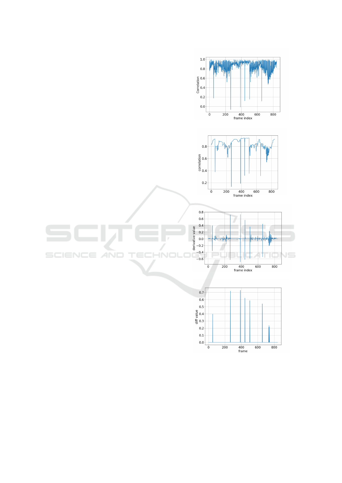
5.2 Query Video Processing
Once a query video is selected, it is processed by
our methodology. Hence, we compute the cross-
correlation through expression (7), shown in Figure
2.(a). Next, the obtained result is processed with
the total variation method (section 3), to obtain the
smoother profile of Figure 2.(b). Then, the differ-
entiation operator is applied with the result shown in
Figure 2.(c). Following, a simple thresholding gives
the result of Figure 2.(d) highlighting the intervals.
In these operations, we use the following parameters
values obtained by trial and error: (1) Total varia-
tion parameters: λ = 0.2 and number of iterations
N
it
= 100; (b) Threshold for differentiation operator
result: T = 0.3 .
The bars observed in Figure 2.(d) define the be-
ginning and the end of each video segment, which
are candidates to be classes in our approach. The
user analyses these segments to identify the correct
classes and performs the labeling of the query video
images. Besides he/she selects a subset (in this case,
60% frames of each identified class) of labeled im-
ages to compose the set X
s
.
(a)
(b)
(c)
(d)
Figure 2: (a) Correlations C
i,i+1
. (b) Total variation filtering
signal (T (C)
i,i+1
) obtained with λ = 0.2 and N
it
= 10. (c)
Visualization of the differentiation operation. (d) Intervals
obtained by thresholding with T = 0.3 the differentiation
result: [1,53], [54,267], [268,389], [390,445], [446, 505],
[506,656], and [657,844].
Video Summarization through Total Variation, Deep Semi-supervised Autoencoder and Clustering Algorithms
319
5.3 Building Unlabeled, Training and
Validation Sets
For each video of the database we randomly take 10%
of samples and assemble these frames in the unla-
beled set X
t
and other 5% to construct a validation
set. We then assemble the labels and unlabeled sets,
X
s
and X
t
, to form the training dataset.
5.4 Autoencoders
The autoencoders were build with the same config-
uration. The architecture had an input layer, five
hidden layers and one output layer, in the sequence:
[3072,1024, 800, 512, 800, 1024, 3072].
To implement the DTML AE we use Tensorflow
and for the common AE the code was performed in
Keras with Tensorflow as background. We did not
implement both in Keras, because Tensorflow is more
friendly to deal with the customized loss function of
DTML AE approach (expression (6)).
For learning rate µ value in Tensorflow DTML
AE, it was adopted µ = 0.001 and for the common
AE it was used the Keras default value.
All parameters were chosen after some experi-
ments, evaluating the reconstruction error evolution.
The configuration above had have the least error in re-
construction in the evaluation. Furthermore, the num-
ber of epochs for training the network was equal to
500 to the common AE and 1000 for DTML AE.
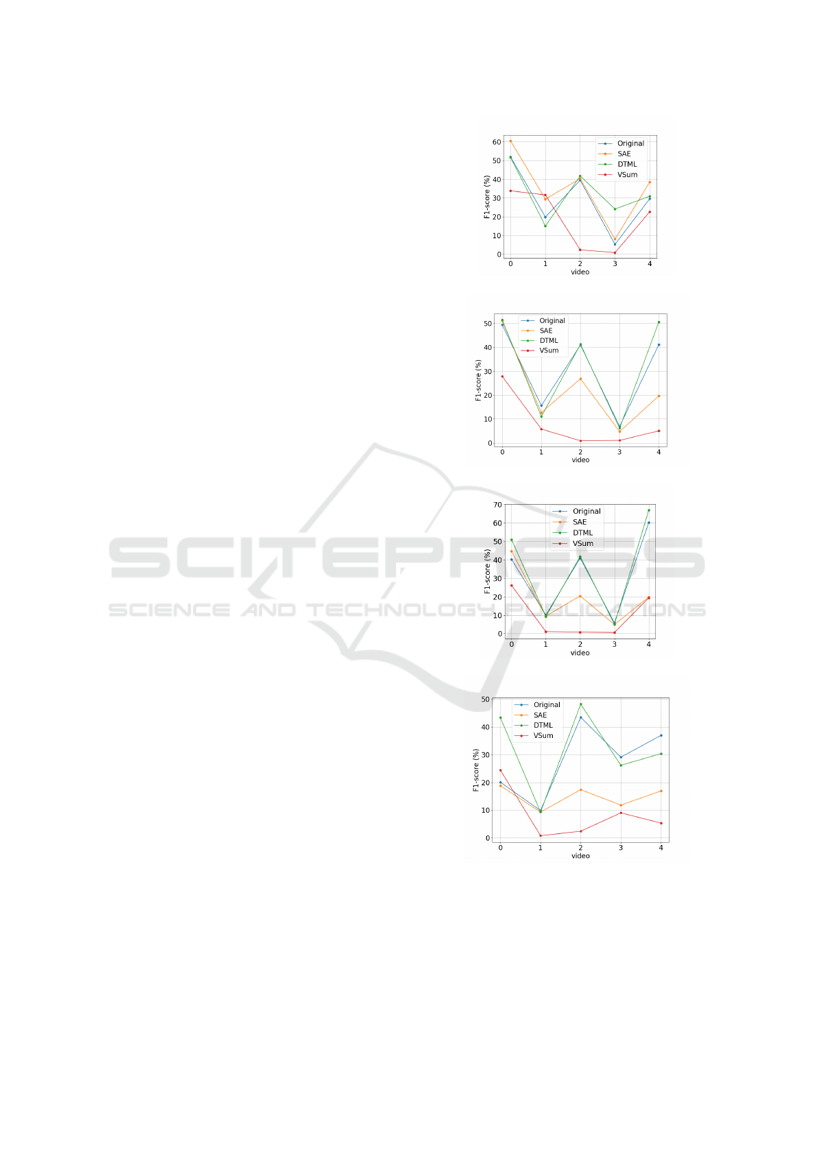
5.5 Test 1
In this test we use five videos from the database for the
final clustering step. This videos were similar to the
query video used to make the X
s
set. The keyframes
were selected based in the proximity with the cluster
centers.
The query video has seven segments, as pointed
by total variation+diff+threshold (results in Figure 2)
and checked in the ground truth. Hence, we set the
number K of clusters to compute the K-means as K ∈
{5,7, 8, 10} in order to test the sensitivity of the F-
score against this parameter. The results are shown in
Figure 3.
We can observe in Figure 3 the mean F-score for
each video and for each space tested, as well as with
different cluster numbers. From this figure we can
observe that DTML AE approach had the higher per-
centile F-score in more videos than the others ap-
proaches. This result is confirmed by the mean per-
centile F-score of all videos as showed in Table 1.
(a) clustering with k=5
(b) clustering with k=7
(c) clustering with k=8
(d) clustering with k=10
Figure 3: Mean F-score for the 30 realizations of k-means
(a) Mean F-score for five test videos using k = 5 clusters;
(b) Mean F-score for five videos using k = 7 clusters; (c)
Mean F-score for five videos using k = 8 clusters (d) Mean
F-score for five videos using k = 10 clusters.
VISAPP 2020 - 15th International Conference on Computer Vision Theory and Applications
320
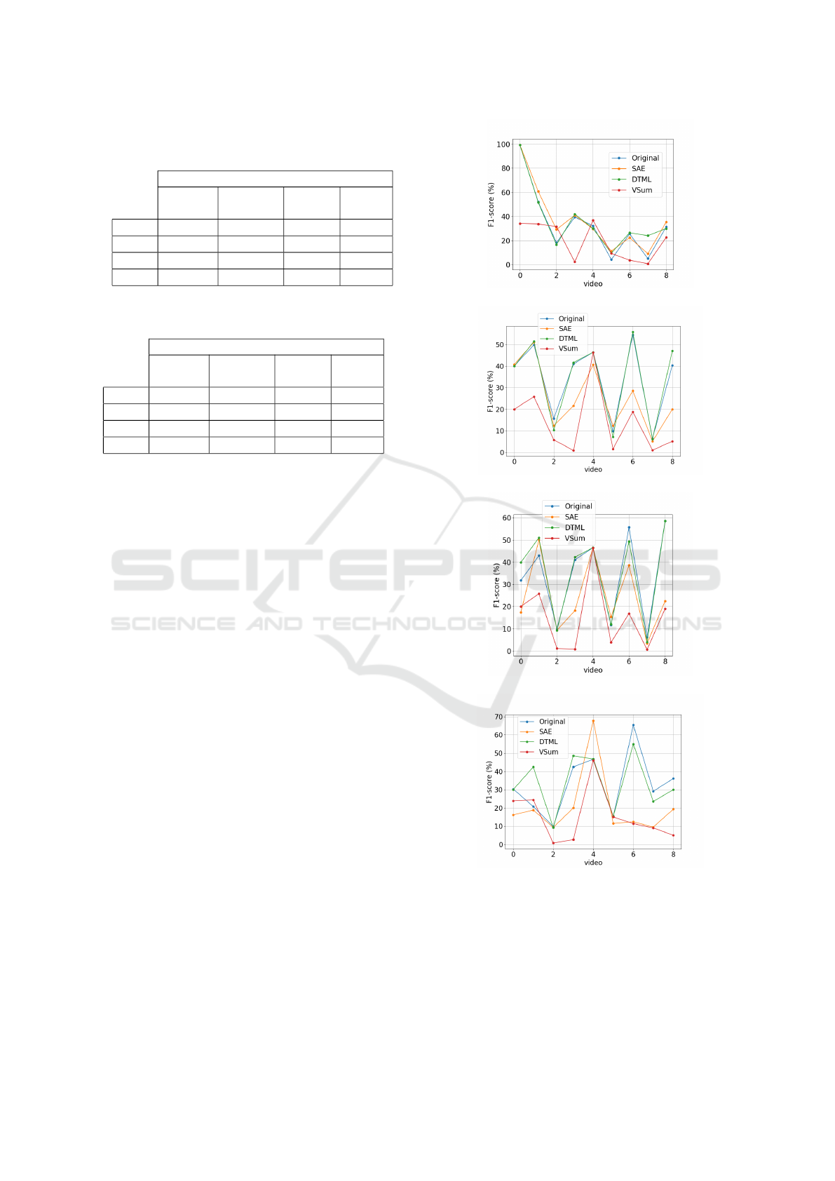
Table 1: F-score for each space varying the clusters number,
using the database with videos similar to the query.
Mean F-score for space
original
common
AE
DTML
AE
VSum
k = 5 0.339 0.258 0.340 0.139
k = 7 0.308 0.230 0.321 0.081
k = 8 0.315 0.199 0.348 0.096
k=10 0.279 0.148 0.315 0.084
Table 2: F-score for each space varying the clusters number.
Considering a database the entire videos.
Space
original
common
AE
DTML
AE
VSum
k = 5 0.342 0.376 0.366 0.195
k = 7 0.338 0.258 0.340 0.139
k = 8 0.338 0.246 0.348 0.150
k=10 0.329 0.205 0.334 0.153
5.6 Test 2
In this test we use all videos from the database for
the final clustering step, in a total of 9 videos. This
database includes videos with different patterns re-
spect to the query video used to make the X
s
set.
It was used the same procedure as the test be-
fore. The results are showed in Figure 4. By the
results shown in Figure 4 we can observe again that
DTML AE approach had the higher percentile F-score
in more videos than the others approaches. This result
is confirmed also by the mean percentile F-score of all
videos reported in Table 2.
6 CONCLUSIONS
In this paper we propose a pipeline to video summa-
rization based on a semi-supervised approach, where
an autoenconder is used to learn a metric space and
the summarization is performed in the encoder space.
The methodology is inspired in the work (Ramos
et al., 2018), originally proposed for fluid summariza-
tion in numerical simulations without computational
experiments reported. We have adapted the method-
ology for video summarization, replacing some ele-
ments of the original pipeline to total variation (TV)
with differentiation and thresholding; cosine similar-
ity; the k-means for clustering. Also, we perform
tests using simple AE, the DTML AE proposed in
(Hu et al., 2016), and compare the methodology re-
sults with the VSum technique.
(a) clustering with k=5
(b) clustering with k=7
(c) clustering with k=8
(d) clustering with k=10
Figure 4: Mean F-score for the 30 realizations of k-means
(a) Mean F-score for five videos using k = 5 clusters; (b)
Mean F-score (%) for five videos using k = 7 clusters; (c)
Mean F-score for five videos using k = 8 clusters (d) Mean
F-score for five videos using k = 10 clusters.
Video Summarization through Total Variation, Deep Semi-supervised Autoencoder and Clustering Algorithms
321

The results showed that the F-score for DTML AE
gives the best result in mean, when compared with
a common AE, the original data space, and VSum
methodology. This result is the same when we con-
sider videos that are similar to the query video, or
when we include videos with low similarity with the
query.
As future works we intent to improve the pipeline
by testing the methodology with convolutional au-
toencoders, using larger datasets for tests and also to
apply a more state of art transformation, as percep-
tual hashing (Monga and Evans, 2006). Moreover,
we want to explore the methodology to content visual
retrieval and to compare the results with more recent
approaches of videos summarization.
ACKNOWLEDGEMENTS
The authors thank to CNPq for support.
REFERENCES
de Avila, S. E. F., ao Lopes, A. P. B., da Luz, A., and
de Albuquerque Ara
´
ujo, A. (2011). Vsumm: A mech-
anism designed to produce static video summaries and
a novel evaluation method. Pattern Recognition Let-
ters, 32(1):56 – 68. Image Processing, Computer Vi-
sion and Pattern Recognition in Latin America.
Fajtl, J., Sokeh, H. S., Argyriou, V., Monekosso, D., and
Remagnino, P. (2018). Summarizing videos with at-
tention.
Goodfellow, I., Bengio, Y., and Courville, A. (2016). Deep
Learning. MIT Press.
Hu, J., Lu, J., Tan, Y.-P., and Zhou, J. (2016). Deep transfer
metric learning. Trans. Img. Proc., 25(12):5576–5588.
Jung, Y., Cho, D., Kim, D., Woo, S., and Kweon, I. S.
(2018). Discriminative feature learning for unsuper-
vised video summarization.
Lei, Z., Zhang, C., Zhang, Q., and Qiu, G. (2019). Framer-
ank: A text processing approach to video summariza-
tion.
Li, X., Li, H., and Dong, Y. (2019). Meta learning for task-
driven video summarization. IEEE Transactions on
Industrial Electronics, 2019.
Mohan, J. and Nair, M. S. (2018). Dynamic summa-
rization of videos based on descriptors in space-time
video volumes and sparse autoencoder. IEEE Access,
6:59768–59778.
Monga, V. and Evans, B. L. (2006). Perceptual image hash-
ing via feature points: Performance evaluation and
tradeoffs. Trans. Img. Proc., 15(11):3452–3465.
Pelleg, D. and Moore, A. W. (2000). X-means: Extend-
ing k-means with efficient estimation of the number
of clusters. In Proc. of the Seventeenth International
Conference on Machine Learning, ICML ’00, pages
727–734, San Francisco, CA, USA.
Ramos, E., da Silva, L., Cardoso, J. S., and Giraldi, G.
(2018). Deep neural network for vector field topology
recognition with applications to fluid flow summariza-
tion.
Rochan, M. and Wang, Y. (2018). Video summarization by
learning from unpaired data.
Rochan, M., Ye, L., and Wang, Y. (2018). Video summa-
rization using fully convolutional sequence networks.
Selesnick, I. (2012). Total variation denoising (an mm algo-
rithm). http://eeweb.poly.edu/iselesni/lecture notes/
TVDmm/TVDmm.pdf. Accessed: 2019-06-10.
Stavropoulos, P. P., Pereira, D., and Kee, H.-Y. (2019). Mi-
croscopic mechanism for higher-spin kitaev model.
Yuan, L., Tay, F. E., Li, P., Zhou, L., and Feng, J. (2019).
Cycle-sum: Cycle-consistent adversarial lstm net-
works for unsupervised video summarization.
Zhao, B., Li, X., and Lu, X. (2019). Hierarchical recurrent
neural network for video summarization.
VISAPP 2020 - 15th International Conference on Computer Vision Theory and Applications
322
