Reﬂective Surface Reconstruction from Inverse Deﬂectometric

Measurements

Dominik Penk

, Roman Sturm

, Lars Seifert

, Marc Stamminger

and G

unther Greiner

Visual Computing Lab, Friedrich-Alexander-Universit

at Erlangen-N

urnberg (FAU), Cauerstraße 11, Erlangen, Germany

Rupp + Hubrach Optik GmbH, Von-Ketteler-Straße 1, Bamberg, Germany

Fraunhofer IIS, Flugplatzstraße 75, F

urth, Germany

marc.stamminger@fau.de

Keywords:

Reconstruction, Quality Control, Simulation, Numerical Optimization.

Abstract:

Reconstructing reﬂective surfaces is a difﬁcult task since most algorithms rely on photometric consistency

between multiple views on the target object. However specular reﬂections are highly view dependent and thus

violate this assumption. Previous work therefore often incorporates additional information, like polarization

or the distortion of a known pattern, to perform specular surface reconstruction. We present a novel analy-

sis by synthesis approach that deﬁnes an optimization problem using samples directly on the reconstructed

surface. Based on this framework we describe two different setups for reconstruction, one using a line laser

to create a reﬂection pattern and a second one, that uses point measurements to provide ray-measurement

correspondences achieving improved accuracy.

1 INTRODUCTION

Above the age of 40 most people develop presbyopia,

an eye disease caused by decreasing ﬂexibility of the

human eye lens. Focusing on close objects becomes

increasingly more difﬁcult. The most common tool to

cope with this kind of defect is wearing glasses with

varying refractive power. There are bifocals, trifo-

cals and, nowadays most popular, so-called progres-

sive addition lenses (PAL). They have a continuously

varying refractive power, lower in the upper part of

the lens (which is typically used to observe distant ob-

jects, e.g. when driving) and higher in the lower part

of the lens (which is usually used for close objects,

e.g. when reading).

The design of such lenses is highly sophisticated

and the resulting geometry of the lens’ surfaces is

rather complex. The manufacturing is complicated

and requires high precision CNC cutting and polish-

ing machines. Quality control is very important, since

small errors in the geometry may lead to high changes

in refractive power. Currently used techniques to

measure PALs have various problems: Either they are

not sufﬁciently accurate, destructive, not fast enough

or require expensive hardware. Therefore, they can-

not be used in a production line to realize a complete

quality control. Furthermore, they either only mea-

sure the curvature of one surface or infer a total lens

power in transmission. For an as worn simulation

however, a surface reconstruction of front and back-

side of the lens is necessary. We set out to develop

an algorithm that directly computes the lens surface

(either front or back face) and derive the optical prop-

erties from there.

In this paper we derive an analysis-by-synthesis

approach to measure lenses based on recreating re-

ﬂection patterns. We present two setups, one using a

line laser. The laser sheet is reﬂected by the lens and

generates a light curve on a screen that is recorded by

a standard camera. Moving the lens through the laser

generates a set of curves that are unique to each sur-

face. We describe a novel optimization scheme, that

from these curves directly reconstructs B-Spline co-

efﬁcients deﬁning the lens surface. Evaluation of this

setup implies that reconstruction accuracy is primar-

ily impeded by the continuous laser line prohibiting a

clear matching of ray to line position. To overcome

this hurdle, we propose the second setup in Sect. 4,

which uses a dot line laser instead of a continuous line

to produce single point measurements. These discrete

points represent a sparser sampling of the reﬂection

pattern, but also introduce a simple mapping from ray

to curve point.

The main contribution of this paper is the in-

Penk, D., Sturm, R., Seifert, L., Stamminger, M. and Greiner, G.

Reﬂective Surface Reconstruction from Inverse Deﬂectometric Measurements.

DOI: 10.5220/0008968600760084

In Proceedings of the 15th International Joint Conference on Computer Vision, Imaging and Computer Graphics Theory and Applications (VISIGRAPP 2020) - Volume 4: VISAPP, pages

76-84

ISBN: 978-989-758-402-2; ISSN: 2184-4321

troduction of an intuitive and efﬁcient optimization

framework that

• directly determines surface parameters,

• has a simple analytic derivation supporting a fast

optimization, and

• is easy to adapt to both setups.

Furthermore, we present results from real world mea-

surements and simulated setups and discuss advan-

tages and drawbacks for both presented setups.

2 RELATED WORK

While there are many well-established methods to

measure/reconstruct surface geometry of diffuse ob-

jects, there are fewer techniques that are applica-

ble to reﬂective or transparent objects. On the one

hand there are contact based methods, so-called Co-

ordinate Measuring Machines (Hocken and Pereira,

2011). The accuracy is satisfactory, but the time for

precise measurements is high. Moreover, high pre-

cision CMMs are very costly. For measuring as-

pheric lenses/PALs optical based methods do a better

job. A common approach is based on interferometry

(Chamadoira et al., ). This method allows measuring

the optical properties/effects of the lens (e.g. spheri-

cal curvature and astigmatism) at speciﬁed points. It

is not possible to recover the actual surface geometry

of the lens. Hence it does not allow variance analysis

during production, i.e. comparing the fabricated lens

with design data and checking compliance of fault

tolerances. Another optical method for measuring is

based on deﬂectometry (Knauer et al., ; Kaminski,

2008; Knauer, 2006; Werling et al., 2007). One or two

cameras capture the mirror image of a regular pattern

(typically a sinusoidal one). Then the methods infer a

normal ﬁeld that leads to the distortion of the regular

pattern. This method is very precise and can recover

the geometry of the reﬂective surface by integration

within reasonable time. When it is applied to PALs,

the back surface must be blackened during the mea-

surement. Clearly, this prohibits the use of the lens

after the measurement, i.e. this method is destructive

and cannot be used in a production line.

The method proposed by (Wedowski et al., 2012)

shares a similar setup to the one we propose, however

an initial reconstruction is required. In a second step

they estimate ﬁner details on the object by estimating

a normal map from the reﬂection pattern.

To specify the geometry of PALs different math-

ematical models are used in the industry. Most pop-

ular are Zernicke polynomials (ZP) and tensor prod-

uct B-Splines. We use the latter description. First

of all because the samples we measured with our

approach where designed accordingly (Loos et al.,

1998). Moreover, to represent lenses with highly

varying refractive power, a ZP of high degree (up

to 20) is required, which causes stability issues for

numeric surface evaluation. Using tensor product B-

splines, the number of control points can be increased

to gain sufﬁcient variability in the geometry, the poly-

nomial degree remains low and surface evaluation is

numerically reliable.

3 LINE MEASUREMENT

3.1 Setup

Our measuring arrangement is depicted in Fig. 1a and

consists of a line laser, a screen and a standard cam-

era. During a scan, we move the measured object

with constant velocity and capture the resulting re-

ﬂection pattern on the screen. For each frame in the

acquired video stream, we detect the reﬂection curve.

To ease the following computations, we assume that

the curve has an explicit representation and ﬁnd the

y-coordinate of the reﬂection curve for each camera

column. We store these values as columns of an im-

age, as depicted in Fig. 1c. The resulting image is

parameterized by the frame index ∆ and the camera

column; pixel values denote the y-coordinate of the

reﬂection curve in frame ∆. We tested our setup with

a variety of different lenses and were always able to

ﬁnd an arrangement that produced such explicit re-

ﬂection curves. We call this new measuring method

Inverse Deﬂectometry referring to the related clas-

sic Deﬂectometry (Knauer et al., ; Kaminski, 2008;

Knauer, 2006; Werling et al., 2007). In contrast to

this method we do not project a dense pattern onto

the measuring object and directly observe the distor-

tion on the surface. We instead capture the reﬂection

pattern on a screen and infer the shape from this in-

direct measurement. This enables us to clearly sepa-

rate the reﬂections from different sides of the lens en-

abling us to conduct a nondestructive measurement.

For the setups presented in this paper we ﬁltered the

camera images to remove backface reﬂections prior

to line extraction. Another important difference is that

our method generates an actual surface reconstruction

whereas the direct deﬂectometirc method produces a

normal ﬁeld.

3.2 Scan Simulation

Our reconstruction method is an analysis-by-

synthesis approach. We use a parametrized geometric

Reﬂective Surface Reconstruction from Inverse Deﬂectometric Measurements

Screen

Laser

Camera

Lens

(a) Measurement setup

Laser Lens Screen Camera

Planar Spotlight Bi-cubic B-spline

Plane Pinhole Camera

(b) Measurement setup sketch

Camera y

Camera x

∆

Measuring step

Figure 1: Subﬁgure (a) depicts the proposed setup. (b) is a sketch of the same setup with annotated parts. In the top row the

real-world objects are listed, on the bottom we show the corresponding models used for simulation. (c) shows an exemplary

result of a measuring drive. The individual measurement steps represent a single column in the image with the y-coordinate

of the reﬂection lines represented by colors.

surface model to simulate the acquisition process

and optimize the surface parameters to reproduce the

presented measurement. We model the screen as a

plane and use an extended pinhole model to simulate

the camera and account for lens distortion during

acquisition by undistorting the camera images before

extracting measurement data.

The surface description is a vital part of the re-

construction and should be chosen carefully to en-

sure a high-quality reconstruction while simultane-

ously retaining decent runtimes. In particular, the

model should require as few codependent parameters

as possible. Besides this, our use case requires that the

mean curvature is well deﬁned on the entire surface.

Based on these preconditions we choose an ex-

plicit uniform bi-cubic B-spline S (Farin, 2002) as the

geometric surface model. S is deﬁned by height val-

ues h

i j

arranged on a regular m × n grid h and two

associated knot-vectors. To form an explicit repre-

sentation of the surface, the knots are chosen such

that the xy-coordinates are always equivalent to uv-

coordinates on the B-spline domain. The z-coordinate

of a surface point is given by a convex combination of

the height values:

S(uv, h) =

∑

i, j

i j

(uv)h

i j

= w(uv)

h (1)

i j

(u,v) is the product of the bi-cubic B-spline basis

functions described in (Farin, 2002). We drop the ar-

guments for brevity if they are unambiguous. Note

that the local support of the B-spline basis functions

implies that only 16 coefﬁcients are nonzero for any

point on the surface. Fig. 1b shows a sketch of the

proposed setup including real world hardware and as-

sociated virtual models used during simulation.

3.3 Optimization

Let R be a subset of all rays emitted by the laser. By

tracing one of these rays r ∈ R through the measuring

setup, using the surface S, parameterized by the con-

trol points h, and a lens offset ∆, we ﬁnd the corre-

sponding simulated measurement q(r, h) on the cam-

era chip. Using this simulation, we can formulate an

intuitive error term:

(h,M) =

∑

r∈R

M(q(r, h)

, ∆) − q(r, h)

(2)

Here M(row,column) is an image access and | · |

is a

stable norm-like function (e.g. Huber-norm).

There are however some major drawbacks to this

formulation. During optimization each ray has to be

intersected with the surface. For a general bi-cubic

B-spline this is most efﬁciently done with an iterative

process, which is still relatively slow, and an analyt-

ical derivation of this process is nontrivial. Finally,

many of the rays may not even hit the surface and

therefore do not add any information to the optimiza-

tion.

We thus propose a novel optimization scheme,

that measures the error by sampling the surface S di-

rectly. Since this is the domain of the optimization

target we will only generate meaningful residuals and

do not waste computation time for ray surface inter-

section. The line laser emits a planar bundle of rays

and we can easily compute the advance ∆ and ray

r, required for simulating the measurement, given a

sample uv on S:

∆(uv) = −

S(uv) + d

(3)

r(uv) = (o

, S(uv) − o

) (4)

Where o

, n

and d

deﬁne the laser and a is the dis-

placement vector of the lens between two consecutive

frames. The error term using surface samples is very

similar to Eq. 2:

(h,M) =

∑

M(q(r, h)

, ∆ − q(r, h)

(5)

VISAPP 2020 - 15th International Conference on Computer Vision Theory and Applications

Lens Ground Truth Reconstruction Error

PAL

−30

−20

−10

v[mm]

−30 0 30

u[mm]

+1.0

+2.0

+3.0

+4.0

Dioptre

−30

−20

−10

v[mm]

−30 0 30

u[mm]

0.0

+0.1

+0.2

+0.3

+0.4

+0.5

+0.6

+0.7

+0.8

Dioptre Error

Spherical

−30

−20

−10

v[mm]

−30 0 30

u[mm]

+3.0

+4.0

+5.0

+6.0

Dioptre

−30

−20

−10

v[mm]

−30 0 30

u[mm]

0.0

+0.1

+0.2

+0.3

+0.4

+0.5

+0.6

+0.7

+0.8

+0.9

+1.0

Dioptre Error

(a) Ground truth error. (b) Simulation error.

Figure 2: (a) displays the divergence of reconstructed and ground truth diopter over the surface. (b) depicts the value of the

objective function without the smoothing term.

Since lenses are smooth, we encourage smooth-

ness by adding the thin plate energy term to the ob-

jective function:

(h) =

Ω

(uv) + 2S

(uv) + S

(uv)

) duv

(6)

Here S

, S

and S

are the second derivatives of the

bi-cubic B-spline S. This energy function is often

used when working with splines, e.g. for mesh fair-

ing (Greiner, 1994) or data approximation (Bookstein,

1989). Combining this regularization with the orig-

inal simulation error yields the ﬁnal objective func-

tion:

argmin

+ λ

(7)

We can solve this optimization problem using

standard nonlinear solvers (e.g. LM (More, 1977))

which require partial derivatives for the objective

function. Eq. 3 is based on ray tracing which is a

recursive method. For each ray intersection we only

require knowledge of the incoming ray and some pa-

rameters speciﬁc to the current intersection (e.g. sur-

face normal for reﬂection or implicit plane equation

for ray-plane intersection). Essentially, the new ray is

given by r

i+1

= f (r

, h) and we can apply the chain

rule to obtain the derivative:

∂r

i+1

∂h

∂ f

∂r

∂h

(8)

To provide all data required for optimization, we

extend the classic ray deﬁnition by the partial deriva-

tives of origin and direction. Eq. 3 implies that the

lens offset ∆ depends on h. We therefore add it to the

ray data leading to a sextuple describing a ray r:

r =



o, d, ∆,

∂o

∂h

∂d

∂h

∂∆

∂h



(9)

Directly sampling the surface implies that the deriva-

tive of the initial ray

∂r

∂h

solely depends on the B-

spline weights w:

∂r

∂h

(uv) = (0, w) (10)

The derivative is constant throughout optimization

and we therefore can precompute the structure of the

sparse Jacobian matrix. This is another advantage of

the proposed sampling strategy over using a ﬁxed set

of rays. If the optimization is set up according to Eq. 2

each residual will produce a different surface sample

in each iteration potentially changing the inﬂuenced

control points and therefore the structure of the Jaco-

bian.

3.4 Results

To demonstrate our method we show the results of

two measured lenses: a simple spherical lens and

a custom designed PAL. Fig. 2a shows the result-

ing deviations from the ground truth captured via

the phase measuring deﬂectometric method (PMD)

(Knauer, 2006). We blacked and roughed the front

faces of the glasses to capture the ground truth. For

the PAL we started optimization from a sphere with

a radius corresponding to the far sight region of the

lens. For the spherical lens we started from a plane.

The presented results show that the optimization

converges to a low simulation error (see Fig. 2b), but

the recovered surface is not sufﬁciently accurate. In

the following we analyze the reasons for this insufﬁ-

cient accuracy.

A major hurdle for most reconstruction methods

based on reﬂection patterns is the height ambiguity,

as described in (Knauer, 2006). The problem is vi-

sualized in Fig. 3: Given a single ray r and its mea-

Reﬂective Surface Reconstruction from Inverse Deﬂectometric Measurements

= n

M(r

)

M(r

)

Figure 3: Depiction of the height problem and how it is

resolved with a parameterized surface. Along a single ray

(e.g. r

) we can always derive a normal to reﬂect it towards

the measurement. For two rays however, there is only one

feasible plane.

surement M(r) we can choose an arbitrary point on r

and derive a normal that reﬂects the ray towards its as-

signed target. This ambiguity is a difﬁcult challenge

for many deﬂectometric methods since the number of

solutions is inﬁnite and the uncoupled ray measure-

ments have to be combined without physical reason-

ing.

Our method, in contrast, by construction intro-

duces plausible dependencies between rays by inter-

secting them with a common surface. Fig. 3 shows

that this implicitly solves the height ambiguity for the

simple case of a planar surface. We need at least two

rays to construct a well determined system since each

ray creates two residuals in Eq. 5 and a plane is de-

ﬁned by four parameters. This reasoning transfers

to bi-cubic B-spline surfaces used in our method, as-

suming that the B-spline is sufﬁciently variable to de-

scribe the actual lens. Since the B-spline represen-

tation has a local support it is important to sample

the entire domain to create a well-deﬁned optimiza-

tion problem. We directly sample the surface to gen-

erate residuals for the optimization and therefore can

ensure this easily.

The second source of ambivalence in our setup

is the matching of rays to point along the measured

curves. Inspecting the simulated reﬂection lines using

the ﬁnal optimization result implies that this is indeed

a major problem. The optimization tends to generate

reﬂection curves that are shorter than the measured

lines and only cover a subsegment. As seen in Fig. 2b

the simulation error still diminishes since Eq. 5 en-

forces that the simulated line is on the measured line

but does not require complete coverage. Experiments

to add an error term to enforce total line coverage

were not successful. We therefore propose to intro-

duce a mapping from rays, produced by the laser, to a

position on the reﬂected line.

(Wedowski et al., 2012) follow a similar idea

where they directly map the simulated to measured

reﬂection. Since they start their reconstruction from

an initial photometric scan, they assume that the sim-

ulation is already very similar to the measurement and

linearly map line segments between distinctive points.

We strife to provide a reconstruction method without

any speciﬁc initial guess. In the following we there-

fore change our ﬁrst setup slightly to provide the ray-

measurement matching directly.

4 DOT LINE MEASUREMENT

4.1 Setup Modiﬁcation

There are many possibilities to introduce ray-

measurement correspondence to the measurement.

We propose to replace the continuous line laser with

a laser producing a dotted line. Many of these lasers

provide a recognizable center ray (e.g. using a big-

ger radius) and we can from there infer the remaining

points by simply counting the distance to the center

ray. The measurement output changes slightly: In-

stead of a height ﬁeld of stacked lines we use an image

of size |dots| × |images| where each entry stores the

pixel position where the corresponding dot is detected

in by camera. See Fig. 4 for an exemplary measure-

ment. We update the simulation error to accommo-

date for the new data:

(h,M) =

∑

d (M(r,∆) − q(r, h)) (11)

Where M(row, column) is once again an image ac-

cess and d(·) is an appropriate distance function (e.g.

squared L

norm). Given this new measurement data

we can now also work with loops, assuming the mea-

surement can handle them, since the pixel coordinates

are now completely separate from the measurement

domain.

The modiﬁed setup replaces continuous line sam-

ples with a discrete sampling of the reﬂection pat-

tern. Therefore, the laser rays, present in the real-

world measurement, also samples the lens surface at

830

Pixel Coordinate

570

X-Coordinate Y-Coordinate

Dot Index

Lens o ﬀ set ∆

Dot Index

Lens oﬀset ∆

Figure 4: An exemplary new measurement with pixel coor-

dinates displayed separately and color-coded.

VISAPP 2020 - 15th International Conference on Computer Vision Theory and Applications

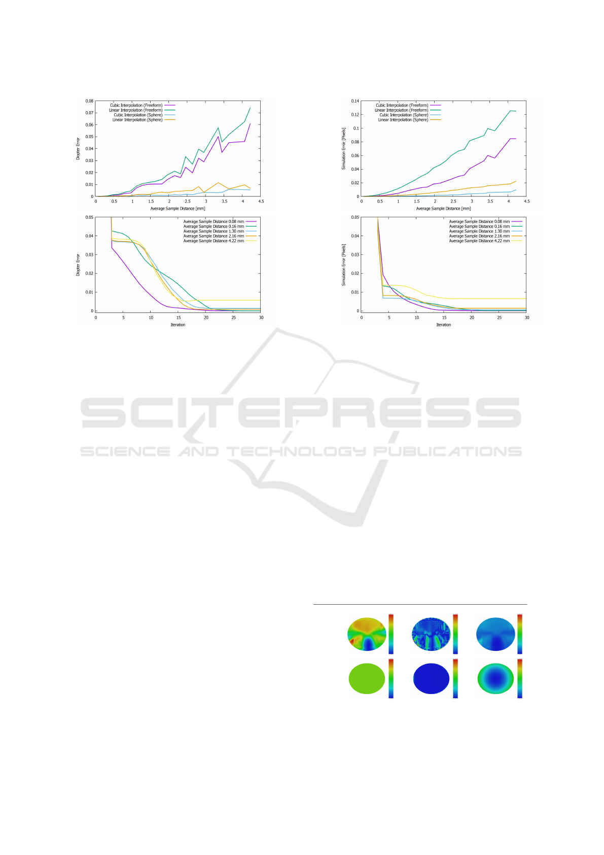
(a) Mean absolute diopter difference to ground truth. (b) Simulation error E

as deﬁned in Eq. 11.

Figure 5: Ground truth and simulation error for a variety of lenses and sample rates.

discrete positions. Our optimization chooses random

points on the spline domain and therefore will fre-

quently trace rays not present in the measurement. To

generate an accurate reconstruction, it is paramount to

ﬁnd a good estimate of the reﬂection pattern for these

unseen rays. Depending on the distance between

consecutive measurement points commonly used lin-

ear interpolation might not be sufﬁcient. We instead

opted for a bicubic interpolation of the measurement

since the reconstructed lenses are very smooth and

therefore also create a smooth reﬂection pattern. As

we will show in the following chapter this interpo-

lation method produces better results, especially for

coarser sample patterns compared to linear interpola-

tion.

4.2 Results

To thoroughly evaluate the behavior of our method

we used a simulated environment where we can easily

test many different parameters of the setup. To eval-

uate the behavior of the reconstruction with different

sampling rates we simulated several PAL designs (de-

noted as freeform) and spherical lenses ranging from

negative to highly positive diopter values. The recon-

struction progress always started from a plane. Re-

sults are summarized in the plots of Fig. 5.

We successively increased the angle between rays

produced by the laser which leads to increasing

spread of scanned points on the lens. The sample dis-

tance ranges from an average of 0.08 mm to 4.22 mm.

As expected, we can use a much wider spread of laser

rays for spherical lenses compared to PALs. For the

latter surfaces we could potentially loose details that

are small enough to ﬁt in the gap between the discrete

data points. Note that the simulation error for PAL

surfaces is generally higher. The reason is twofold,

ﬁrst the smoothing term Eq. 6 prevents overﬁtting to

the measurement. On the other hand, the reﬂection

curve produced by a PAL is less smooth in compari-

son to a spherical lens resulting in a larger interpola-

tion error.

Fig. 6 shows some exemplary reconstructions

starting from a plane. The sample rate was chosen

to generate an average dot sample distance of 2mm.

Larger deviations from the ground truth are primar-

ily located at fringes of the lens. To represent the

entire lens surface with the B-spline, we chose a do-

main larger than the actual lens and cut out the spher-

Lens Ground Truth Reconstruction Error Thinplate Error

PAL

Spherical

Figure 6: Reconstruction results for exemplary lenses. The

reconstruction error ist the absolute difference to the ground

truth and clamped to 0.1 dioptre.

Reﬂective Surface Reconstruction from Inverse Deﬂectometric Measurements

ical shape. This implies that fewer residuals are cre-

ated for control points near the border of the lens

and the smoothing term has a larger inﬂuence lead-

ing to worse reconstruction. However real measure-

ments tend to create very noisy and inaccurate mea-

surements near the edge of the lens. These error result

from inter reﬂections or rough surface on the edges,

such that we decided not to reduce the inﬂuence of

the smoothing term towards the fringes.

As mentioned in Sect. 4.1 we assume that the

interpolation of the sparse measurements has a pro-

found impact on the ﬁnal reconstruction. To ver-

ify this, we compared the bicubic and bilinear inter-

polation of M for different sample rates. The ﬁrst

method results in a smooth function even at pixel bor-

ders, whereas the linear interpolation can cause G1-

discontinuities. The top plot in Fig. 5a shows that the

bicubic interpolation is generally the superior interpo-

lation method especially for freeform surfaces with a

lower sample rate. For higher sample rates however,

the linear interpolation is also a good approximation.

Finally, we study the convergence rate of the op-

timization procedure in the second row of Fig. 5.

The simulation and ground truth error behave simi-

lar and only change insigniﬁcantly for the ﬁrst ﬁfteen

to twenty iterations for the simulated objects.

5 CONCLUSION AND FUTURE

WORK

We presented two setups to reconstruct a lens sur-

face from its reﬂection pattern. We have shown that

a continuous line, used in the ﬁrst setup, produces

reconstructions of inadequate accuracy for quality

control. However, the proposed optimization frame-

work and setup was adapted to explicitly provide

ray-measurement correspondences. The optimiza-

tion framework is agnostic to the actual measurement

technique, if a mapping from the surface point to the

space of the light source is available. In future work

we will try different types of lasers that directly en-

code the angle along the ray (e.g. using phase encod-

ing) and evaluate if the denser measurements signiﬁ-

cantly impact reconstruction quality.

In this paper we explicitly ﬁltered secondary re-

ﬂections to stick to a simple light path with a single

reﬂection at the initial surface. We therefore require

two scans to fully capture a single lens. The presented

framework can be extended easily to more complex

paths with multiple surface interactions. We will in-

corporate this into our method to simultaneously cap-

ture both sides of a PAL in a single measurement.

Although the reconstruction time of around 2 min-

utes is short enough to include the method as a qual-

ity assurance tool into an existing production line, we

would like to speed up the process. Since the simula-

tions of the individual laser rays, done during residual

computation, are independent, we anticipate a mean-

ingful speedup by implementing a GPU based version

of our algorithm.

ACKNOWLEDGEMENTS

This research is funded by Bayerische Forschungss-

tiftung ”Schritthaltende 3D-Rekonstruction und -

Analys (AZ-1184-15)” (For3D). The lenses and PALs

are provided by our project partners Rupp+Hubrach

Brillenglas.

REFERENCES

Agarwal, S., Mierle, K., and Others. Ceres solver.

http://ceres-solver.org.

ohm, W. (1977). Cubic b-spline curves and surfaces

in computer aided geometric design. Computing,

19(1):29–34.

Bookstein, F. L. (1989). Principal warps: thin-plate splines

and the decomposition of deformations. IEEE Trans-

actions on Pattern Analysis and Machine Intelligence,

11(6):567–585.

Chamadoira, S., Blendowske, R., and Acosta, E. Progres-

sive addition lens measurement by point diffraction in-

terferometry. OPTOMETRY AND VISION SCIENCE,

89(10):15321542.

Farin, G. (2002). Curves and Surfaces for CAGD: A Prac-

tical Guide. Morgan Kaufmann Publishers Inc., San

Francisco, CA, USA, 5th edition.

Greiner, G. (1994). Variational Design and Fairing of Spline

Surfaces. Computer Graphics Forum, 13(3):143–154.

Halstead, M. A., Barsky, B. A., Klein, S. A., and Mandell,

R. B. (1996). Reconstructing curved surfaces from

specular reﬂection patterns using spline surface ﬁtting

of normals. In Proceedings of the 23rd Annual Con-

ference on Computer Graphics and Interactive Tech-

niques, SIGGRAPH ’96, pages 335–342, New York,

NY, USA. ACM.

Hocken, R. and Pereira, P. (2011). Coordinate Measuring

Machines and Systems, Second Edition. CRC Press.

Kaminski, J. (2008). Geometrische Rekonstruktion spiegel-

nder Oberﬂ

achen aus deﬂektometrischen Messdaten.

PhD thesis, FAU Erlangen N

urnberg.

Kaminski, J., Lowitzsch, S., Knauer, M. C., and H

ausler, G.

(2006). Full-ﬁeld shape measurement of specular sur-

faces. In Osten, W., editor, Fringe 2005, pages 372–

379, Berlin, Heidelberg. Springer Berlin Heidelberg.

Knauer, M. (2006). Absolute Phasenmessende Deﬂektome-

trie. PhD thesis, FAU Erlangen N

urnberg.

VISAPP 2020 - 15th International Conference on Computer Vision Theory and Applications

Knauer, M., Kaminski, J., and H

ausler, G. Phase measur-

ing deﬂectometry: a new approach to measure specu-

lar free-form surfaces. In editor, editor, Proceedings

of SPIE - The International Society for Optical Engi-

neering, volume 5457.

Loos, J., Greiner, G., and Seidel, H.-P. (1998). A variational

approach to progressive lens design. Computer-Aided

Design, 30(8):595 – 602.

More, J. (1977). Levenberg–marquardt algorithm: imple-

mentation and theory. Numerical analysis, 630.

Moreno, D. and Taubin, G. (2012). Simple, accurate, and

robust projector-camera calibration. In 2012 Second

International Conference on 3D Imaging, Modeling,

Processing, Visualization Transmission, pages 464–

471.

Rahmann, S. and Canterakis, N. (2001). Reconstruction

of specular surfaces using polarization imaging. In

Proceedings of the 2001 IEEE Computer Society Con-

ference on Computer Vision and Pattern Recognition.

CVPR 2001, volume 1, pages I–149–I–155 vol.1.

Richter, C., Kurz, M., Knauer, M., and Faber, C. (2009).

Machine-integrated Measurement of Specular Free-

formed Surfaces Using Phase-measuring Deﬂectom-

etry, vol. 6. EUSPEN 2009.

Sorkine, O. (2005). Laplacian Mesh Processing. In

Chrysanthou, Y. and Magnor, M., editors, Eurograph-

ics 2005 - State of the Art Reports. The Eurographics

Association.

Tan, C.-T., Chan, Y.-S., Lin, Z.-C., and Chiu, M.-H. (2011).

Angle-deviation optical proﬁlometer. Chin. Opt. Lett.,

9(1):011201.

Wang, S.-W., Shih, Z.-C., and Chang, R.-C. (2002). An ef-

ﬁcient and stable ray tracing algorithm for parametric

surfaces. J. Inf. Sci. Eng., pages 541–561.

Wedowski, R., Atkinson, G., Smith, M., and Smith, L.

(2012). Dynamic deﬂectometry: A novel approach

for the on-line reconstruction of specular freeform sur-

faces. Optics and Lasers in Engineering, 50:1765–

1778.

Werling, S., Balzer, J., and Beyerer, J. (2007). A new ap-

proach for specular surface reconstruction using de-

ﬂectometric methods. In Informatik 2007 - Informatik

trifft Logistik. Bd.1. Hrsg.: R. Koschke, volume 109 of

GI-Edition / Proceedings, pages 44–48. Gesellschaft

ur Informatik, Bonn.

APPENDIX

The integral part of our reconstruction method is trac-

ing a single ray through the acquisition geometry and

the derivative of this path according to the B-spline

height values h. In this appendix we present the for-

mulas and derivatives needed to construct most paths

present in a real-world setup. We will use the short-

hand f

for

∂ f

∂x

for brevity in this appendix.

Both reﬂection and refraction require the nor-

malised normal at a point (u,v) on the B-spline do-

main. The normal is easily derived since we chose an

explicit version of the B-spline:

n =



−S







−S





(12)

We deﬁne l =





−S





, w

and w

are

the derivatives of the B-spline basis functions with re-

spect to the indices.









l +









+ S

)

(13)

After a surface intersection the incoming ray i ei-

ther refracts into the surface (t) or gets reﬂected (r)

as shown in Fig. 7. In reality both cases will occur

but since only the shape of the resulting pattern is of

interest, we deﬁne a ﬁx interaction type during opti-

mization. The cosine of the incident angle and its’

derivation is given by

cos(θ

) = −i

cos(θ

)

= −i

− n

(14)

From this the reﬂection direction is easily computed:

r = i + 2 cos(θ

= i

+ 2(cos(θ

)

n + cos(θ

)

(15)

The refractive indices of the two neighboring media at

the surface are needed to compute the refraction ray,

Figure 7: Refraction and Reﬂection.

Reﬂective Surface Reconstruction from Inverse Deﬂectometric Measurements

which has the following form:

t =

i +



cos(θ

) −

1 − sin

(θ

)







cos(θ

)

sin

(θ

)

1 − sin

(θ

)







cos(θ

) −

1 − sin

(θ

)



(16)

with

sin

(θ

) =





(1 − cos

(θ

))

sin

(θ

)

= −2





cosθ

cos(θ

)

(17)

After the ray interacted with the lens, we have to

model the ﬁnal two steps along the light path. The

ﬁrst one is the point on the screen deﬁned by the plane

p + d

= 0 (18)

where n

and p a point on the plane. If we insert a

point on the ray r into this equation we can compute

the intersection point s:

s = o − αd

= o

− dα

+ α − d

α =

o + d

)(n

d) − (n

o + d

)(n

)

(19)

The ﬁnal projection onto the camera image plane q

and subsequent dehomogenisation is given by:

q = KTs

= KTs

q =



q.x q.y



q.z

q =

q.z



.x q



−



q.x q.y



q.z

(20)

Where the camera intrinsics K and extrinsics T are

known. q.x refers to the x-component of the vector q

(equivalent for y and z)

VISAPP 2020 - 15th International Conference on Computer Vision Theory and Applications