
Information Preserving Discriminant Projections
Jing Peng
1
and Alex J. Aved
2
1
Department of Computer Science, Montclair State University, Montclair, NJ 07043, U.S.A.
2
Information Directorate, AFRL, Rome, NY 13441, U.S.A.
Keywords:
Classification, Dimensionality Reduction, Feature Selection.
Abstract:
In classification, a large number of features often make the design of a classifier difficult and degrade its
performance. This is particularly pronounced when the number of examples is small relative to the number
of features, which is due to the curse of dimensionality. There are many dimensionality reduction techniques
in the literature. However, most these techniques are either informative (or minimum information loss), as
in principal component analysis (PCA), or discriminant, as in linear discriminant analysis (LDA). Each type
of technique has its strengths and weaknesses. Motivated by Gaussian Processes Latent Variable Models, we
propose a simple linear projection technique that explores the characteristics of both PCA and LDA in latent
representations. The proposed technique optimizes a regularized information preserving objective, where
the regularizer is a LDA based criterion. And as such, it prefers a latent space that is both informative and
discriminant, thereby providing better generalization performance. Experimental results based on a variety of
data sets are provided to validate the proposed technique.
1 INTRODUCTION
In machine learning, a large number of features or
attributes often make the development of classifiers
difficult and degrade their performance. This is par-
ticularly pronounced when the number of examples
is small relative to the number of features, which is
due to the curse of dimensionality (Bellman, 1961).
It simply states that the number of examples required
to properly compute a classifier grows exponentially
with the number of features. For example, assuming
features are correlated, approximating a binary distri-
bution in a d dimensional feature space requires es-
timating O(2
d
) unknown variables (Breiman et al.,
1984).
Many machine learning problems are fundamen-
tally related to the problem of learning latent rep-
resentations or subspace learning, which potentially
benefits many applications (Banerjee and Peng, 2005;
Peng, 1995; Heisterkamp et al., 2000; ?). The goal of
subspace learning is to discover the geometric prop-
erties of the input space, such as its Euclidean embed-
ding, intrinsic dimensionality, and connected compo-
nents from a set of high dimensional examples. Sub-
space learning is also related to embedding. Subspace
learning techniques can be categorized into linear and
non-linear techniques. In this paper, we are mainly
interested in linear techniques for simplicity and re-
duced computational complexity.
There are many dimensionality reduction tech-
niques in the literature (Belhumeur et al., 1997; Fuku-
naga, 1990; Huo and et al, 2003; Howland and Park,
2004; Peng et al., 2013; Aved et al., 2017; Zhang
et al., 2005). However, most these techniques are ei-
ther informative (or minimum information loss), as
in principal component analysis (PCA), or discrimi-
nant, as in linear discriminant analysis (LDA). Each
type of technique has its strengths and weaknesses.
For example, PCA is unsupervised, while LDA is su-
pervised. Thus, it seems that in classification, LDA
should be able to outperform PCA. However, it has
been shown that PCA can outperform LDA in classi-
fication problems, given insufficient training data per
subject (Martinez and Kak, 2001).
Motivated by Gaussian Processes (GP) latent
variable models (Lawrence, 2005; Rasmussen and
Williams, 2005; Urtasun and Darrell, 2007) and local-
ity preserving projections (He and Niyogi, 2003; Cai
et al., 2006), we investigate linear projection models
that exploit the characteristics of PCA and LDA in
latent representations. The latent representation com-
puted by PCA is most informative in terms of min-
imum information loss. On the other hand, it does
not take into account class label information. Thus,
162
Peng, J. and Aved, A.
Information Preserving Discriminant Projections.
DOI: 10.5220/0008967601620171
In Proceedings of the 12th International Conference on Agents and Artificial Intelligence (ICAART 2020) - Volume 2, pages 162-171
ISBN: 978-989-758-395-7; ISSN: 2184-433X
Copyright
c
2022 by SCITEPRESS – Science and Technology Publications, Lda. All rights reserved

it is less discriminant in general. By combining the
characteristics of both PCA and LDA, it is expected
that the resulting latent can be both informative and
discriminant, thereby providing better generalization
performance. Experimental results using a variety of
data sets are provided to validate the proposed tech-
nique.
2 RELATED WORK
Many techniques have been proposed to take the ad-
vantage of the inherent low dimensional nature of the
data (Darnell et al., 2017; Harandi et al., 2017; Sarve-
niazi, 2014; Xie et al., 2017). Two major linear sub-
space learning techniques are PCA and LDA. Both
are capable of discovering the intrinsic geometry of
the latent subspace. However, they only compute the
global Euclidean structure.
Linear techniques based on graph Laplacians such
as locality preserving projections (LPP) can model
the local structure of the latent subspace (He and
Niyogi, 2003). These techniques construct an adja-
cency matrix that captures the local geometry of the
latent space from class label information. The pro-
jections are then computed by preserving such an ad-
jacency structure. However, the basis functions ob-
tained from LPP are not guaranteed to be orthogonal,
which makes the data reconstruction more difficult.
Orthogonal LPP (OLPP) is a linear dimension re-
duction technique that has been proposed to address
the problems associated with LPP (Cai et al., 2006).
Similar to LPP, OLPP computes an adjacency ma-
trix that preserves locality information. On the other
hand, OLPP computes its basis functions that are
guaranteed to be orthogonal, Orthogonal basis func-
tions preserve the metric structure of the latent space.
It is shown OLPP outperforms LPP (Cai et al., 2006).
GP latent variable models are probabilistic tech-
niques for computing low dimensional subspaces
from high dimensional data (Gao et al., 2011;
Lawrence, 2005; Urtasun and Darrell, 2007; Jiang
et al., 2012). These techniques have been applied to
many problems such as image reconstruction and fa-
cial expression recognition (Abolhasanzadeh, 2015;
Cai et al., 2016; Eleftheriadis et al., 2015; Song et al.,
2015a).
GP latent variable models are generativeand com-
pute a latent subspace without taking into account
class label information, as in (Lawrence, 2005). They
are useful for visualization and regression analysis.
And as such, the resulting latent space may not be op-
timal for classification. One way to address this prob-
lem is to introduce a prior distribution such as the uni-
form prior over the latent space to place constraints on
the resulting latent space (Urtasun and Darrell, 2007).
One of the main problems associated with GP latent
variable models is that for a given test example, a sep-
arate estimation process must take a place to compute
the corresponding latent position. This inference in-
troduces additional uncertainties in the entire GP la-
tent variable model computation and added computa-
tional complexity.
Integrating PCA and LDA for dimension reduc-
tion has been discussed in the literature (Yu et al.,
2007; Zhao et al., 2011). These techniques formulate
an objective as a linear combination of PCA and LDA
criteria. On the other hand, we optimize the PCA ob-
jective with LDA as regularizer. This regularization
view has a well established foundation in Gaussian
Process latent variable models.
3 GAUSSIAN PROCESS LATENT
VARIABLE MODELS
Gaussian Process (GP) latent variable models com-
pute a low dimensional latent representation of high
dimensional input data, using a GP mapping from the
latent space to the input data space. Here we briefly
describe GP latent variable models to motivate the in-
troduction of the proposed technique.
Let
X = [x
1
,x
2
,··· ,x
n
]
t
be a set of centered data, where x
i
∈ ℜ
d
, and t denotes
the transpose operator. Also, let
Z = [z
1
,z
2
,· ·· ,z
n
]
t
represent the corresponding latent variables, where
z
i
∈ ℜ
q
, and q ≪ d. A typical relationship between
the two sets of variables can be described by
x = Wz+ ε, (1)
where W is a d × q matrix, and ε denotes the error
term. Assuming that p(ε) = N(0,β
−1
I) (i.e., isotropic
Gaussian), we have the following conditional proba-
bility distribution over the input space
p(x|z,W,β) = N(Wz,β
−1
I).
This implies that the likelihood of the data can be
written as (matrix normal distribution)
p(X|Z,W,β) =
n
∏
i=1
p(x
i
|z
i
,W,β).
Here it is assumed that x
i
are independent and iden-
tically distributed (i.i.d.). Probabilistic PCA solution
Information Preserving Discriminant Projections
163

for W can be computed by integrating out the latent
variables (Tipping and Bishop, 1999).
A dual approach is to integrate out W and opti-
mize the latent variables (Lawrence, 2005; Urtasun
and Darrell, 2007). First, we specify a prior distri-
bution p(w
i
) = N(0,α
−1
I) for W, where w
i
is the ith
row of W. Then
p(W) =
d
∏
i=1
p(w
i
) =
1
C
d
exp(−
1
2
tr(αW
t
W))
=
α
dq
2
(2π)
dq
2
exp(−
1
2
tr(αW
t
W)). (2)
where C
d
is a normalization constant. Therefore, the
marginalized likelihood of X can be computed by in-
tegrating out W
p(X|Z,β) =
Z
p(X|Z,W,β)p(W)dW
∝
1
|K|
d/2
exp(−
1
2
tr(K
−1
XX
t
)), (3)
where
K = (α
−1
ZZ
t
+ β
−1
I).
Thus, the distribution of the data given the latent vari-
ables is Gaussian. It can be shown that the solution
Z, obtained by maximizing the GP likelihood of the
latent variables (3), is equivalent to the PCA solution
(Lawrence, 2005; Tipping and Bishop, 1999).
One can place additional conditions on the latent
variables Z by introducing priors over Z. For exam-
ple, if we place a uniform prior on Z, the log prior
becomes
ln p(Z) = −
1
2
n
∑
i=1
z
t
i
z
i
.
Such a prior prefers the latent variables close to the
origin (Urtasun and Darrell, 2007). In classification
context, one can incorporate class labels into the prior
(Eleftheriadis et al., 2015; Song et al., 2015b). This
can be accomplished based on discriminant analy-
sis (Fukunaga, 1990). For example, LDA J(Z) =
tr(S
−1
w
S
b
), where S
w
and S
b
denote the between and
within class matrices in the latent space, can be im-
posed. Here tr denotes the matrix trace. The prior
thus becomes (Urtasun and Darrell, 2007)
p(Z) = Cexp(−J
−1
).
One of drawbacks associated with GP latent mod-
els is that for a given test example, a separate esti-
mation process must take a place to compute the cor-
responding latent position. This inference introduces
additional uncertainties in the entire GP latent model
computation and added computational complexity.
4 INFORMATION PRESERVING
DISCRIMINANT
PROJECTIONS
In this section, we develop a novel algorithm that
combines some of the best features of Gaussian Pro-
cess latent models and locality preserving projections.
As discussed above, the optimization of the likeli-
hood (3) results in the PCA solution to the latent vari-
ables Z in the GP latent models. By introducing priors
over latent variables p(Z), one obtains the log poste-
rior (terms that the posterior depends on)
L = −
d
2
ln|K| −
1
2
tr(K
−1
XX
t
) + lnp(Z). (4)
As noted in (Rasmussen and Williams, 2005; Urtasun
and Darrell, 2007), in a non-Bayesian setting, the log
prior ln p(Z) can be viewed as a penalty term. And
the maximum a posterior estimate of the latent vari-
ables can be interpreted as the penalized maximum
likelihood estimate. If one introduces a discriminant
prior, (4) represents a trade-off between informative
(as in PCA) and discriminant (as in LDA) representa-
tions. A major drawback is that a separate estimation
process must take place for each test example.
To overcome this problem, we introduce a simple
linear projection technique that preserves the repre-
sentation balance shown in (4), without a separate in-
ference process for test examples. Recall that PCA
finds the projection p by maximizing
J(p) = tr(p
t
XX
t
p), (5)
where XX
t
denotes the covariance matrix, assuming
the data are centered. Projection p has the property
that the loss
n
∑
i
kx
i
− pp
t
x
i
k
2
is minimum. Thus, PCA solutions are entirely infor-
mational in that the resultinglatent representation pre-
serves the maximum information.
To encourage the latent space to be discriminant,
we appeal to the idea behind GP latent variable mod-
els, where the prior over the latent variables place
constraints on variable positions in the latent space.
As noted above, the log prior can be simply inter-
preted as a regularizer. Along this line, we can in-
troduce a regularizer in (5)
J(p) = tr(p
t
XX
t
p) + λr(p), (6)
where r(·) represents a regularizer and λ is the reg-
ularization constant. r(·) plays the role of the log
prior in GP latent models that places a constraint in
the resulting latent space. In this work, we introduce
the following regularizers: Laplacian and Linear Dis-
criminant Analysis (LDA).
ICAART 2020 - 12th International Conference on Agents and Artificial Intelligence
164

4.1 Information Preserving Projections
with Laplacian Regularizer
A locality preserving projection (LPP) builds a graph
of the input data that preserves local neighborhoodin-
formation (He and Niyogi, 2003). LPP then computes
a linear projection from the Laplacian of the graph.
Let W be a n× n weight matrix, where
W
ij
=
exp(−tkx
i
− x
j
k
2
) i 6= j and l(x
i
) = l(x
j
)
0 otherwise.
(7)
Here x
i
represents the ith training example, l(·) de-
notes the label of its input, and t is a kernel parameter.
Let p be a projection such that z
i
= p
t
x
i
. LLP com-
putes a linear projection by minimizing the following
ojective
∑
i, j
(z
i
− z
j
)
2
W
ij
.
A penalty is incurred when examples x
i
and x
j
that
are in the same class are projected far apart. It turns
out that the above objective can be rewritten as
1
2
∑
i, j
(z
i
− z
j
)
2
W
ij
=
1
2
∑
i, j
(p
t
x
i
− p
t
x
j
)
2
W
ij
= p
t
X
t
LXp, (8)
where L = D− W is the graph Laplacian, and D is
a diagonal matrix with diagonal entries D
ii
=
∑
j
W
ij
.
Since D
ii
indicates the volume of z
i
, LLP places the
following constraint on the objective
min
p
p
t
X
t
LXp (9)
s.t. p
t
X
t
DXp = 1
The optimal solution can be obtained by solving the
generalized eigenvalue problem
X
t
LXp = λX
t
DXp. (10)
LPP has been shown to be effective in practice (He
and Niyogi, 2003; Cai et al., 2006).
In LPP (He and Niyogi, 2003), the optimal projec-
tion p is computed by minimizing p
t
X
t
LXp. There-
fore, the proposed Laplacian regularized PCA be-
comes
J(p) = tr(p
t
XX
t
p) + λtr(p
t
(X
t
LX)
−1
p). (11)
Thus, p can be computed by maximizing
J
IP−Lap
= tr(XX
t
+ λ(X
t
LX)
−1
). (12)
We call the resulting projection Information Preserv-
ing Laplacian Projection, or PLap. Note that (11) can
be interpreted as a regularized PCA, where LPP is the
regularizer. Or it can be viewed as a regularized LPP,
where the regularizer is PCA.
4.2 Information Preserving Projections
with LDA Regularizer
We can similarly introduce the LDA regularizer
J(p) = tr(p
t
XX
t
p) + λtr(p
t
S
−1
w
S
b
p), (13)
where
S
w
=
C
∑
c=1
n
c
∑
i=1,x
i
∈c
(x
i
− m
c
)(x
i
− m
c
)
t
and
S
b
=
C
∑
c=1
(m
c
− m)(m
c
− m)
t
are the between-class and within-class matrices. Here
m represents the overall mean, m
c
denotes the mean
of class c, and t represents the transpose operator.
Projection p can be computed by maximizing
J
IP−LDA
= tr(XX
t
+ λS
−1
w
S
b
). (14)
We call the resulting projection Information Preserv-
ing LDA Projection, or PLda. Similar to PLap (11),
(13) can be interpreted as a regularized PCA, where
LDA is the regularizer. Or it can be viewed as a regu-
larized LDA, where the regularizer is PCA.
5 EXPERIMENTS
We now examine the performance of the proposed
techniques against competing techniques using sev-
eral examples.
5.1 Methods
The following methods are evaluated in the experi-
ments.
1. PLap–Information Preserving Projection with
Laplacian regularizer (Eq. 12).
2. PLda–Information Preserving Projection with
LDA regularizer (Eq. 14).
3. PCA–Projection that maximizes (Eq. 5)
J(p) = tr(p
t
XX
t
p).
4. LDA–Projection that maximizes
J(p) = tr((p
t
S
w
p)
−1
p
t
S
b
p),
where S
w
and S
b
are the within and between ma-
trices, respectively.
5. OLPP–Orthogonal Laplacian Projection (OLPP)
proposed in (Cai et al., 2006).
Information Preserving Discriminant Projections
165
-3 -2 -1 0 1 2 3
-1.5
-1
-0.5
0
0.5
1
1.5
2
-3 -2 -1 0 1 2 3
-1.5
-1
-0.5
0
0.5
1
1.5
2
-3 -2 -1 0 1 2 3
-0.6
-0.4
-0.2
0
0.2
0.4
0.6
-3 -2 -1 0 1 2 3
-0.6
-0.4
-0.2
0
0.2
0.4
0.6
0.8
-0.4 -0.3 -0.2 -0.1 0 0.1 0.2 0.3 0.4
-0.6
-0.4
-0.2
0
0.2
0.4
0.6
-0.5 -0.4 -0.3 -0.2 -0.1 0 0.1 0.2 0.3 0.4
-1
-0.8
-0.6
-0.4
-0.2
0
0.2
0.4
0.6
0.8
-0.4 -0.3 -0.2 -0.1 0 0.1 0.2 0.3 0.4
-0.6
-0.4
-0.2
0
0.2
0.4
0.6
-0.5 -0.4 -0.3 -0.2 -0.1 0 0.1 0.2 0.3 0.4
-0.8
-0.6
-0.4
-0.2
0
0.2
0.4
0.6
0.8
-1.5 -1 -0.5 0 0.5 1 1.5 2
-2
-1.5
-1
-0.5
0
0.5
1
1.5
-1.5 -1 -0.5 0 0.5 1 1.5 2
-2
-1.5
-1
-0.5
0
0.5
1
1.5
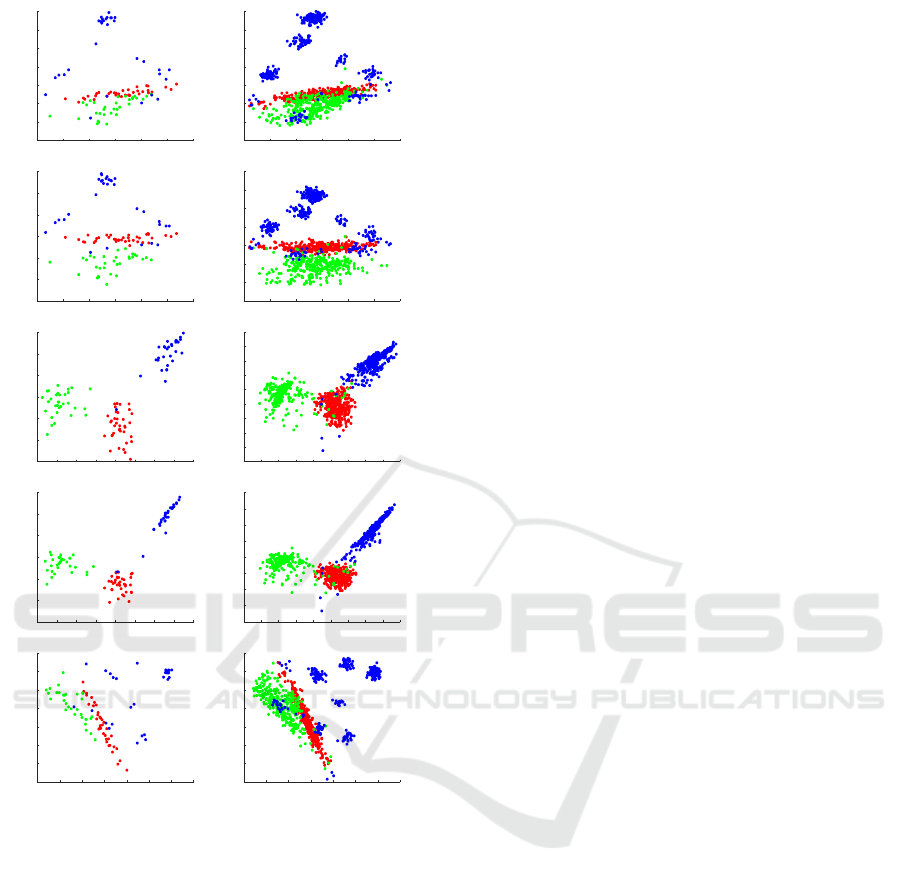
Figure 1: Oil flow data projected onto two dimensional
spaces. The left column (top to bottom) shows the two di-
mensional representation of the training examples by PCA,
LDA, PLap, PLda, and OLPP, respectively. The right col-
umn shows the two dimensional representation of the test
examples by PCA, PLap, PLda, LDA, and OLPP, respec-
tively.
Note that OLPP is along the line of LPP (9). It is
known that the solution to (10) may not be orthogonal.
To address this problem, OLPP first projects the data
onto the PCA subspace, where it computes the solu-
tion to (10) that preserves orthogonality. It is shown
in (Cai et al., 2006) OLPP outperformsLPP. Thus, we
compare the proposed technique against OLPP in our
experiments.
5.2 Oil Flow Data
We have carried out an experiment to visually exam-
ine our proposed techniques. The data set is the multi-
phase oil flow data (Bishop and James, 1993). This
data set contains examples in 12 dimensions. The data
set has three classes corresponding to the phase of
flow in an oil pipeline: stratified, annular and homo-
geneous. In this experiment, for illustration purposes,
we randomly sampled 100 examples as the training
data, and additional 1000 examples as the test data.
Figure 1 shows the two dimensional projections
by the five competing techniques. The left column
(top to bottom) shows the two dimensional repre-
sentation of the training examples by PCA, LDA,
PLap, PLda, and OLPP, respectively. The right col-
umn shows the two dimensional representation of the
test examples by the corresponding techniques. For
PLap and PLda, regularization constant λ was to 100.
Kernel parameter t in Laplacian (9) was set to 0.01
for both PLap and OLPP. The plots show that the
proposed techniques provided better class separation
than the competing methods in the latent space.
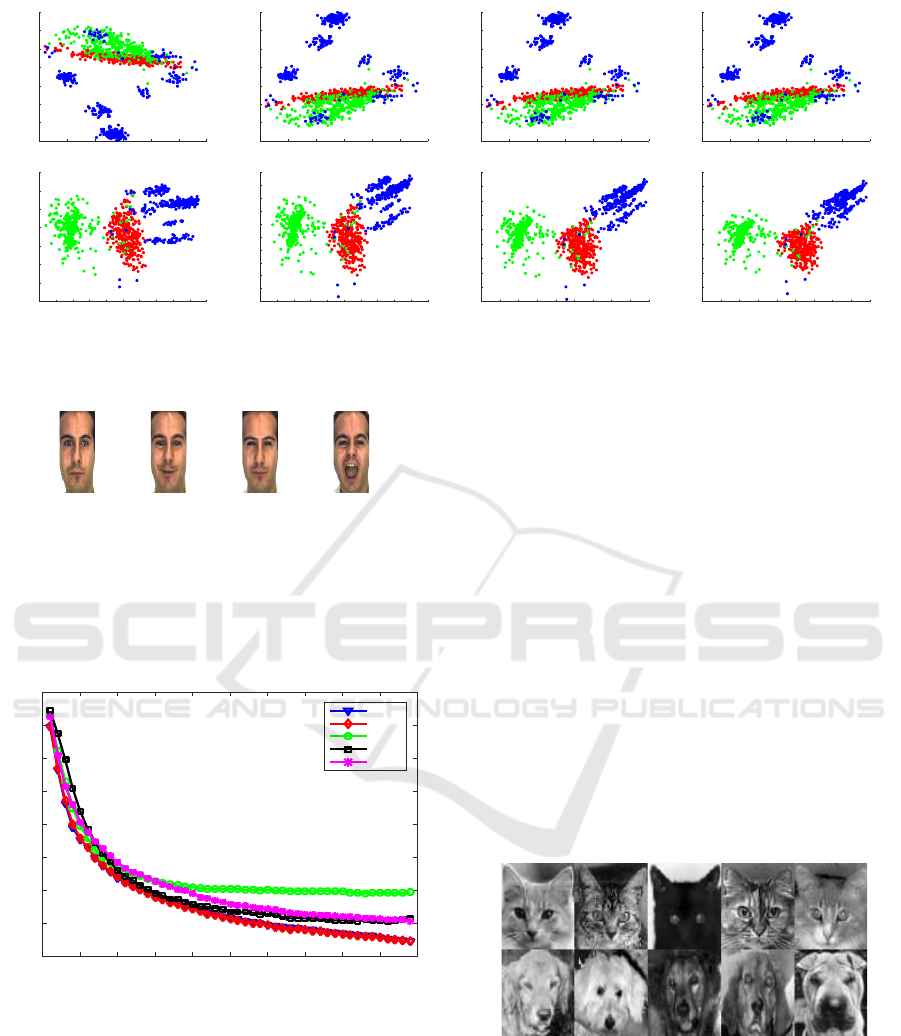
Figure 2 shows two dimensional projections of the
test examples by PLap and PLda as a function of reg-
ularization constant λ: 20, 40, 60, and 80. The top
panel shows the representation by PLap, and the bot-
tom panel shows the representation by PLda. As λ in-
creases, the resulting latent space becomes more dis-
criminant. That is, as λ varies, the latent representa-
tions show the characteristics from PCA to LDA, as
expected.
5.3 AR Face Data
This experiment involves the AR-face database (Mar-
tinez and Kak, 2001). The precise nature of the data
set is described in (Martinez and Kak, 2001). For this
experiment, 50 different subjects (25 males and 25
females) were randomly selected from this database.
Images were normalized to the final 85 × 60 pixel ar-
rays. Sample images are shown in Figure 3.
This experiment follows the exact setup of the
Small Training Data set experiment described in
(Martinez and Kak, 2001), whereit is shown that PCA
can outperform LDA, given insufficient training data
per subject. Here we want to see how the proposed
techniques fare against PCA in such situations.
In this setup, the first seven images from each sub-
ject are selected, resulting in a total of 350 images. To
highlight the effects of a small training data set, two
images from each subject are used as training and the
remaining five are used as testing. Following (Mar-
tinez and Kak, 2001), we use all 21 different ways of
ICAART 2020 - 12th International Conference on Agents and Artificial Intelligence
166
-3 -2 -1 0 1 2 3
-2
-1.5
-1
-0.5
0
0.5
1
1.5
-3 -2 -1 0 1 2 3
-1.5
-1
-0.5
0
0.5
1
1.5
2
-3 -2 -1 0 1 2 3
-1.5
-1
-0.5
0
0.5
1
1.5
2
-3 -2 -1 0 1 2 3
-1.5
-1
-0.5
0
0.5
1
1.5
2
-0.5 -0.4 -0.3 -0.2 -0.1 0 0.1 0.2 0.3 0.4 0.5
-2
-1.5
-1
-0.5
0
0.5
1
1.5
-0.5 -0.4 -0.3 -0.2 -0.1 0 0.1 0.2 0.3 0.4 0.5
-1.2
-1
-0.8
-0.6
-0.4
-0.2
0
0.2
0.4
0.6
0.8
-0.5 -0.4 -0.3 -0.2 -0.1 0 0.1 0.2 0.3 0.4
-1
-0.8
-0.6
-0.4
-0.2
0
0.2
0.4
0.6
0.8
-0.5 -0.4 -0.3 -0.2 -0.1 0 0.1 0.2 0.3 0.4
-1
-0.8
-0.6
-0.4
-0.2
0
0.2
0.4
0.6
0.8
Figure 2: Two dimensional representation of the test examples by PLap and PLda as a function of regularization parameter λ:
20, 40, 60 and 80. The top panel shows the representation by PLap, and the bottom panel shows the representation by PLda.
As λ increases, the resulting latent space becomes more discriminant.
Figure 3: AR sample images.
partitioning the data into training and testing for the
results reported here. The original images of 85× 60
pixels are first transformed via PCA into a space of
350 dimensions spanned by the 350 face data. All the
methods see their input from this space.
Dimensions
0 5 10 15 20 25 30 35 40 45 50
Average Error Rate
0.2
0.3
0.4
0.5
0.6
0.7
0.8
0.9
1
PLap
PLda
LDA
OLPP
PCA
Figure 4: Average error rate registered by PLap, PLda,
LDA, OLPP, and PCA with increasing dimensionality on
the AR face data.
The average error rates in a subspace with 49 di-
mensions over the 21 runs are shown in the first row
in Table 1. Figure 4 plots the average error rates reg-
istered by the competing methods over 21 runs on the
AR face data as a function of increasing dimensions.
On average both PLap and PLda clearly outperform
PCA across the 49 subspaces, and consistently per-
form better than the competing methods.
5.4 Additional Data Sets
Additional data sets are used to illustrate the general-
ization performance by each competing technique.
1. MNIST Data (MNIST). The MNIST dataset con-
sists of handwritten digits from the US National
Institute of Standards and Technology (NIST)
(yann.lecun.com/exdb/mnist/). Each digit is a 28
by 28 pixels of intensity values. Thus each digit is
a feature vector of 784 intensities. In this exper-
iment, we randomly selected 100 examples from
each digit, for a totla of 1000 examples.
2. Cat and Dog data (CatDog). This image data set
consists of two hundred images of cat and dog
faces. Each image is a black-and-white 64 × 64
pixel image, and the images have been registered
by aligning the eyes. Sample cat and dog images
are shown in Figure 5.
Figure 5: Sample images of the cat and dog data.
3. Multilingual Text (MText). This data set is a mul-
tilingual text data set (Amini et al., 2009). It is
from the Reuters RCV1 and RCV2 collections.
The data set consists of six categories of docu-
ments: 1) Economics, 2) Equity Markets, 3) Gov-
ernment Social, 4) Corporate/Industrial, 5) Per-
formance, and 6) Government Finance. Each doc-
ument in English has a corresponding document
Information Preserving Discriminant Projections
167
in French, German, Italian and Spanish, translated
using PORTAGE (Ueffing et al., 2007). The doc-
uments in English are used in this experiment,
where each document is represented by a bag of
words model in 21531 dimensions. In this exper-
iment, we randomly selected 100 examples from
each class. Thus, the data set has 600 examples in
21531 dimensions.
4. Iris Data (Iris). The iris data set is a publicly
available WVU multimodal data set (Crihalmeanu
et al., 2007). The data set consists of iris images
from subjects of different age, gender, and eth-
nicity, as described in (Crihalmeanu et al., 2007).
The data set is difficult because many examples
are low quality due to blur, occlusion, and noise.
Sample iris images are shown in 6. The evaluation
was done on a randomly selected pair of subjects,
where one subject has 27 examples, and the other
subject has 36 examples for a total of 63 exam-
ples.
To compute features, iris images are segmented
into 25 × 240 templates (Pundlik et al., 2008).
Since Gabor features have been shown to pro-
duce better representation for iris data (Daugman,
2004), these templates are convolved with a log-
Gabor filter at a single scale to obtain a 6000 fea-
tures.
Figure 6: Sample Iris images.
5. Fingerprint Data (Finger). Similar to the iris
data set, the finger data set is obtained from pub-
licly available WVU multimodal data sets (Cri-
halmeanu et al., 2007). The data set consists of
fingerprint images from a randomly chosen pair
of subjects. Again, the data set is difficult because
many examples are low quality due to blur, oc-
clusion, and noise. Sample fingerprint images are
shown in 7. This data set has 124 examples, where
one subject has 61 instances, while the other has
63. To represent fingerprints, ridge and bifurca-
tion features are computed using publically avail-
able code (sites.google.com/site/athisnarayanan/).
Resulting feature vectors have 7241 components.
Figure 7: Sample fingerprint images.
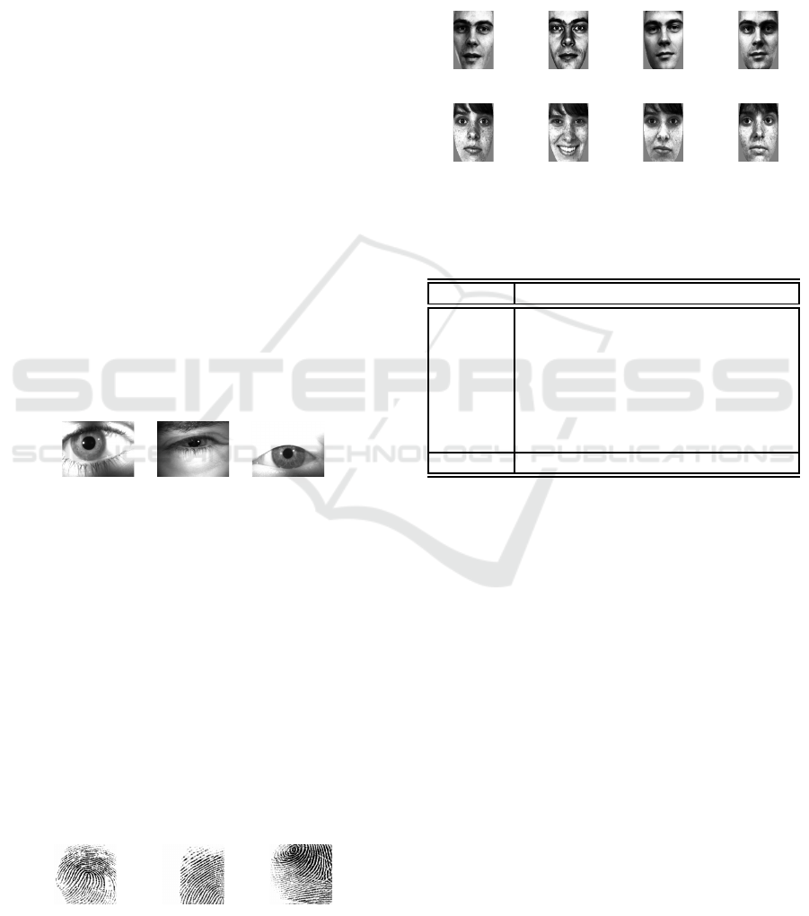
6. Feret Face Data (FeretFace). The FERET face
data set consists of 50 subjects, randomly cho-
sen from the Feret face database (Phillips, 2004).
Each subject has 8 instances. Therefore, we have
a set of 400 facial images. The images used here
involvevariations in facial expressionsand illumi-
nation. Each image has 150× 130 pixels. Sample
images are shown in Figure 8.
Figure 8: Normalized Feret sample images.
Table 1: Average error rates registered by the competing
methods on the 7 data sets.
PCA PLap PLda LDA OLPP
ARFace 0.307 0.245 0.245 0.394 0.314
MNIST 0.143 0.152 0.143 0.402 0.148
CatDog 0.492 0.216 0.210 0.457 0.286
MText 0.405 0.217 0.232 0.365 0.305
Iris 0.480 0.133 0.133 0.141 0.136
Finger 0.466 0.378 0.387 0.444 0.467
FeretFace 0.088 0.042 0.042 0.092 0.098
Ave 0.340 0.198 0.199 0.328 0.251
5.5 Experimental Results
In the additional six data set experiments, all training
data have been normalized to have zero mean and unit
variance along each dimension. The test data are sim-
ilarly normalized using training mean and variance.
In the resulting latent space, the one nearest neighbor
rule is used to perform classification. The regulariza-
tion constant λ and the kernel parameter t in Lapla-
cian (9) were chosen through five fold cross valida-
tion. Table 1 shows the 10-fold crossed validated er-
ror rates of the five competing methods on the 6 data
sets described above.
The table shows that on average both PLap and
PLda outperformed all the competing techniques ex-
amined here. And PLap and PLda performed simi-
larly on these data sets. The results show that classi-
fication performed in a space that is both informative
and discriminant provides better generalization per-
formance than in either the PCA or LDA subspace
alone.
ICAART 2020 - 12th International Conference on Agents and Artificial Intelligence
168
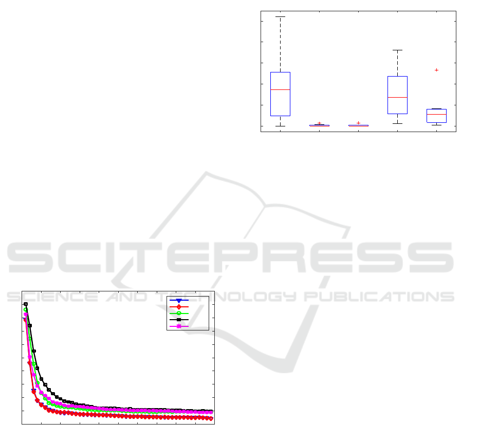
Figure 9 plots the 10-fold error rates computed by
each method on the Feret face data as a function of in-
creasing dimensions. As can be seen, both PLap and
PLda consistently outperform the competing meth-
ods across the 49 subspaces, again demonstrating that
classification performed in a space that is both infor-
mative and discriminant provides better generaliza-
tion performance.
5.6 Robustness of Performance
PLap and PLda clearly achieved the best or near best
performance over the 7 data sets, followed by OLPP.
It seems natural to ask the question of robustness.
That is, how well a particular method m performs on
average in situations that are most favorable to other
methods. We compute robustness by computing the
ratio b
m
of its error rate e
m
and the smallest error rate
over all methods being compared in a particular ex-
ample:
b
m
= e
m
/ min
1≤k≤5
e
k
.
Thus, the best method m
∗
for that example has b
m
∗
=
1, and all other methods have larger values b
m
≥ 1,
for m 6= m
∗
. The larger the value of b
m
, the worse
the performance of the mth method is in relation to
the best one for that example. The distribution of the
b
m
values for each method m over all the examples,
therefore, seems to be a good indicator of robustness.
Dimensions
0 5 10 15 20 25 30 35 40 45 50
Average Error Rate
0
0.1
0.2
0.3
0.4
0.5
0.6
0.7
0.8
0.9
1
PLap
PLda
LDA
OLPP
PCA
Figure 9: Average error rate registered by PLap, PLda,
LDA, OLPP, and PCA with increasing dimensionality on
the Feret face data.
Figure 10 plots the distribution of b
m
for each
method over the 7 data sets. The dark area represents
the lower and upper quartiles of the distribution that
are separated by the median. The outer vertical lines
show the entire range of values for the distribution.
It is clear that the most robust method over the data
sets are PLap. In 5/7 of the data its error rate was the
best (median = 1.0). In the worst case it was no worse
than 62.9% higher than the best error rate. This is fol-
lowed by PLda. In the worst case PLda was no worse
than 69.1%. In contrast, PCA has the worst distribu-
tion, where the worst case was 360.9% higher than
the best error rate.
PCA PLap PLda LDA OLPP
1
1.5
2
2.5
3
3.5
Figure 10: Error distributions of PCA, PLap, PLda, LDA,
and OLPP over the 7 data sets.
6 SUMMARY
We have developed information preserving linear dis-
criminant projections for computing latent represen-
tations. The proposed technique exploits the charac-
teristics of PCA, LDA, and graph Laplacian to com-
pute latent representations that are both informative
and discriminant. As a result, the proposed technique
provides better generalization performance. Experi-
mental results are provided that validate the proposed
technique. We note that the proposed technique is lin-
ear. We plan on extending this technique to the non-
linear case by incorporating kernel tricks in our future
work.
REFERENCES
Abolhasanzadeh, B. (2015). Gaussian process latent vari-
able model for dimensionality reduction in intrusion
detection. In 2015 23rd Iranian Conference on Elec-
trical Engineering, pages 674–678.
Amini, M., Usunier, N., and Goutte, C. (2009). Learning
from multiple partially observed views-an application
to multilingual text categorization. In Advances in
Neural Information Processing Systems, pages 28–36.
Aved, A., Blasch, E., and Peng, J. (2017). Regular-
ized difference criterion for computing discriminants
for dimensionality reduction. IEEE Transactions on
Aerospace and Electronic Systems, 53(5):2372–2384.
Banerjee, B. and Peng, J. (2005). Efficient learning of
multi-step best response. In Proceedings of the Fourth
International Joint Conference on Autonomous Agents
Information Preserving Discriminant Projections
169

and Multiagent Systems, AAMAS ’05, pages 60–66,
New York, NY, USA. ACM.
Belhumeur, V., Hespanha, J., and Kriegman, D. (1997).
Eigenfaces vs. fisherfaces: Recognition using class
specific linear projection. IEEE Transaction on Pat-
tern Analysis and Machine Intelligence, 19(7):711–
720.
Bellman, R. E. (1961). Adaptive Control Precesses: A
Guided Tour. Princeton University Press.
Bishop, C. and James, G. (1993). Analysis of mul-
tiphase flows using dual-energy gamma densitome-
try and neural networks. Nuclear Instruments and
Methods in Physics Research Section A: Accelerators,
Spectrometers, Detectors and Associated Equipment,
327(2):580–593.
Breiman, L., Friedman, J. H., Olshen, R. A., and Stone,
C. J. (1984). Classification and Regression Trees.
Wadsworth and Brooks, Monterey, CA.
Cai, D., He, X., Han, J., and Zhang, H. (2006). Orthogonal
laplacianfaces for face recognition. Trans. Img. Proc.,
15(11):3608–3614.
Cai, L., Huang, L., and Liu, C. (2016). Age estima-
tion based on improved discriminative gaussian pro-
cess latent variable model. Multimedia Tools Appl.,
75(19):11977–11994.
Crihalmeanu, S., Ross, A., Schukers, S., and Hornak, L.
(2007). A protocol for multibiometric data acqui-
sition, storage and dissemination. In Technical Re-
port, WVU, Lane Department of Computer Science
and Electrical Engineering.
Darnell, G., Georgiev, S., Mukherjee, S., and Engelhardt, B.
(2017). Adaptive randomized dimension reduction on
massive data. Journal of Machine Learning Research,
18(140):1–30.
Daugman, J. (2004). How iris recognition works. IEEE
Trans. on Circuits and Systems for Video Technology,
14(21):21–30.
Eleftheriadis, S., Rudovic, O., and Pantic, M. (2015).
Discriminative shared gaussian processes for multi-
view and view-invariant facial expression recognition.
IEEE Transactions on Image Processing, 24(1):189–
204.
Fukunaga, K. (1990). Introduction to statistical pattern
recognition. Academic Press.
Gao, X., Wang, X., Tao, D., and Li, X. (2011). Super-
vised gaussian process latent variable model for di-
mensionality reduction. IEEE Transactions on Sys-
tems, Man, and Cybernetics, Part B (Cybernetics),
41(2):425–434.
Harandi, M., Salzmann, M., and Hartley, R. (2017). Joint
dimensionality reduction and metric learning: A ge-
ometric take. In Precup, D. and Teh, Y. W., edi-
tors, Proceedings of the 34th International Conference
on Machine Learning, volume 70, pages 1404–1413,
International Convention Centre, Sydney, Australia.
PMLR.
He, X. and Niyogi, P. (2003). Locality preserving projec-
tions. In Proceedings of the 16th International Con-
ference on Neural Information Processing Systems,
NIPS’03, pages 153–160. MIT Press.
Heisterkamp, D., Peng, J., and Dai, H. (2000). Feature rele-
vance learning with query shifting for content-based
image retrieval. In Proceedings 15th International
Conference on Pattern Recognition. ICPR-2000, vol-
ume 4, pages 250–253.
Howland, P. and Park, H. (2004). Generalizing discriminant
analysis using the generalized singular valuke decom-
position. IEEE Transactions on Pattern Analysis and
Machine Intelligence, 26(8):995–1006.
Huo, X. and et al (2003). Optimal reduced-rank quadratic
classiers using the fukunaga-koontz transform, with
applications to automated target recognition. In Proc.
of SPIE Conference.
Jiang, X., Gao, J., Wang, T., and Zheng, L. (2012). Su-
pervised latent linear gaussian process latent variable
model for dimensionality reduction. IEEE Transac-
tions on Systems, Man, and Cybernetics, Part B (Cy-
bernetics), 42(6):1620–1632.
Lawrence, N. (2005). Probabilistic non-linear principal
component analysis with gaussian process latent vari-
able models. J. Mach. Learn. Res., 6:1783–1816.
Martinez, A. M. and Kak, A. (2001). Pca versus lda.
IEEE Trans. Pattern Analysis and Machine Intelli-
gence, 23(2):228–233.
Peng, J. (1995). Efficient memory-based dynamic program-
ming. In Proceedings of the Twelfth International
Conference on Machine Learning, pages 438–446.
Peng, J., Seetharaman, G., Fan, W., and Varde, A. (2013).
Exploiting fisher and fukunaga-koontz transforms in
chernoff dimensionality reduction. ACM Transactions
on Knowledge Discovery from Data, 7(2):8:1–8:25.
Phillips, P. (2004). The facial recognition technology (feret)
database. IEEE Trans. Pattern Analysis and Machine
Intelligence, 22.
Pundlik, S., Woodard, D., and Birchfield, S. (2008). Non-
ideal iris segmentation using graph cuts. In IEEE Con-
ference on Computer Vision and Pattern Recognition
Workshops, pages 1–6.
Rasmussen, C. and Williams, C. (2005). Gaussian Pro-
cesses for Machine Learning (Adaptive Computation
and Machine Learning). The MIT Press.
Sarveniazi, A. (2014). An actual survey of dimensionality
reduction. American Journal of Computational Math-
ematics, 4(2):55–72.
Song, G., Wang, S., Huang, Q., and Tian, Q. (2015a).
Similarity gaussian process latent variable model for
multi-modal data analysis. In 2015 IEEE Interna-
tional Conference on Computer Vision (ICCV), pages
4050–4058.
Song, G., Wang, S., Huang, Q., and Tian, Q. (2015b).
Similarity gaussian process latent variable model for
multi-modal data analysis. In 2015 IEEE Interna-
tional Conference on Computer Vision (ICCV), pages
4050–4058.
Tipping, M. and Bishop, C. (1999). Probabilistic princi-
pal component analysis. JOURNAL OF THE ROYAL
STATISTICAL SOCIETY, SERIES B, 61(3):611–622.
Ueffing, N., Simard, M., Larkin, S., and Johnson, J. (2007).
NRC’s PORTAGE system for WMT 2007. In In ACL-
2007 Second Workshop on SMT, pages 185–188.
ICAART 2020 - 12th International Conference on Agents and Artificial Intelligence
170

Urtasun, R. and Darrell, T. (2007). Discriminative gaus-
sian process latent variable model for classification. In
Proceedings of the 24th International Conference on
Machine Learning, ICML ’07, pages 927–934, New
York, NY, USA. ACM.
Xie, P., Deng, Y., Zhou, Y., Kumar, A., Yu, Y., Zou, J.,
and Xing, E. (2017). Learning latent space mod-
els with angular constraints. In Precup, D. and Teh,
Y. W., editors, Proceedings of the 34th International
Conference on Machine Learning, volume 70 of Pro-
ceedings of Machine Learning Research, pages 3799–
3810, International Convention Centre, Sydney, Aus-
tralia. PMLR.
Yu, J., Tian, Q., Rui, T., and Huang, T. S. (2007). Inte-
grating discriminant and descriptive information for
dimension reduction and classification. IEEE Trans-
actions on Circuits and Systems for Video Technology,
17(3):372–377.
Zhang, P., Peng, J., and Domeniconi, C. (2005). Kernel
pooled local subspaces for classification. IEEE Trans-
actions on Systems, Man, and Cybernetics, Part B
(Cybernetics), 35(3):489–502.
Zhao, N., Mio, W., and Liu, X. (2011). A hybrid pca-lda
model for dimension reduction. In The 2011 Inter-
national Joint Conference on Neural Networks, pages
2184–2190.
Information Preserving Discriminant Projections
171
