
Mosaic Images Segmentation using U-net
Gianfranco Fenu
a
, Eric Medvet
b
, Daniele Panfilo and Felice Andrea Pellegrino
c
Dipartimento di Ingegneria e Architettura, Universit
`
a degli Studi di Trieste, Trieste, Italy
Keywords:
Cultural Heritage, Computer Vision, Deep Learning, Convolutional Neural Networks.
Abstract:
We consider the task of segmentation of images of mosaics, where the goal is to segment the image in such a
way that each region corresponds exactly to one tile of the mosaic. We propose to use a recent deep learning
technique based on a kind of convolutional neural networks, called U-net, that proved to be effective in seg-
mentation tasks. Our method includes a preprocessing phase that allows to learn a U-net despite the scarcity
of labeled data, which reflects the peculiarity of the task, in which manual annotation is, in general, costly. We
experimentally evaluate our method and compare it against the few other methods for mosaic images segmen-
tation using a set of performance indexes, previously proposed for this task, computed using 11 images of real
mosaics. In our results, U-net compares favorably with previous methods. Interestingly, the considered meth-
ods make errors of different kinds, consistently with the fact that they are based on different assumptions and
techniques. This finding suggests that combining different approaches might lead to an even more effective
segmentation.
1 INTRODUCTION AND
RELATED WORKS
Cultural heritage is one of the most important assets
of the society. Its preservation and restoration are
time-consuming activities performed by experts and
often consist in manual analysis of fine details of the
works. It is hence natural that these tasks, as many
others where human experts are involved in some
form of data processing, are subjected to automa-
tion using machine learning techniques. Differently
than other domains, however, tasks concerning cul-
tural heritage may be harder because of the scarcity
of labeled data and nature of the data itself. Despite
these limitations, successful examples of applications
exist, e.g., (Assael et al., 2019), and progresses in the
techniques for different kinds of data pave the way for
other successful applications.
In this work we consider a particular kind of artis-
tic works, i.e., mosaics. Mosaics are assemblies of
small pieces of stone or similar materials, called tiles
or tessellae, glued together with some binder or filler,
such that the overall appearance of the assembly looks
like a painting or some decorative pattern. Mosaics
a
https://orcid.org/0000-0003-0867-8388
b
https://orcid.org/0000-0001-5652-2113
c
https://orcid.org/0000-0002-4423-1666
constitute an essential component of the cultural her-
itage for many (ancient) civilizations. Preservation,
and, to some degree, restoration of mosaics might be
enhanced if digital versions of the works were avail-
able. Moreover, the access to the artistic works might
be eased using digital means, possibly as part of a pro-
cess in which hard copies are obtained starting from
digital copies, hence enlarging the portion of popula-
tion that can access mosaics, regardless of their phys-
ical location (Neum
¨
uller et al., 2014). There have
been a couple of approaches, namely (Youssef and
Derrode, 2008; Bartoli et al., 2016), that proposed
automatic methods for obtaining a digital version of
the mosaic. All of them take as input an image of
the mosaic, that can be cheaply obtained also for not-
relocable mosaics, and output a segmentation of the
image in which regions should correspond to tiles.
Starting from the segmentation, a digital version of
the mosaic may be obtained straightforwardly, hence
easing the mosaic preservation and restoration and
making it more accessible (Comes et al., 2014).
Here we propose a novel technique for mosaic im-
age segmentation that is based on a recently proposed
kind of convolutional neural networks (CNN), called
U-net (Ronneberger et al., 2015). Our approach dif-
fers from the previous ones in the way the mosaic im-
age is processed. The U-net processes the image at
the pixel level, differently than the proposal by Bartoli
Fenu, G., Medvet, E., Panfilo, D. and Pellegrino, F.
Mosaic Images Segmentation using U-net.
DOI: 10.5220/0008967404850492
In Proceedings of the 9th International Conference on Pattern Recognition Applications and Methods (ICPRAM 2020), pages 485-492
ISBN: 978-989-758-397-1; ISSN: 2184-4313
Copyright
c
2022 by SCITEPRESS – Science and Technology Publications, Lda. All rights reserved
485

et al. (2016), but permits, by design, that some pixels
are not associated with any region, differently than the
approach of Youssef and Derrode (2008): this means
that using U-net for segmentation allows to model the
presence of the filler. A key component of our ap-
proach is in the preprocessing phase that is part of the
learning process: we propose a method for augment-
ing the dataset in such a way that the learning of U-net
parameters is effective even when a small number of
annotated examples are available. In facts, manual
annotating mosaic images is a costly process (Bartoli
et al., 2016).
We assess experimentally our approach applying
it to 11 images of real mosaics, differing in style, age,
and quality (both of the image and of the mosaic it-
self in terms of wear). We compare the segmentation
based on U-net against previous methods using a set
of established performance indexes suitable for the
mosaic image segmentation task and we found that
our method outperforms the other ones in the most
relevant index. Moreover, we show that the way in
which the three methods make errors in analyzing the
image varies consistently with the fact that the meth-
ods are based on different underlying assumptions.
This finding opens an opportunity for designing an
even more effective method where U-net segmenta-
tion is a step of a more complex procedure which in-
volves also other processing steps, eventually result-
ing in a better segmentation effectiveness.
Despite the availability of a “digital model” could
be very useful, in the literature only few segmenta-
tion algorithms have been proposed, taking into ac-
count the specific structure features of a mosaic, i.e.,
shape, organisation, color of tiles, and the presence
of the filler. In particular, in (Youssef and Derrode,
2008) the proposed approach aims to detect and to
extract the tile from the filler, using the well-known
watershed algorithm (Vincent and Soille, 1991) and
some mosaic-specific preprocessing. In (Bartoli et al.,
2016) the authors proposal goal is the same, but they
employed deformable models as flexible shapes to be
superimposed on the mosaic picture and to be adapted
to the effective shapes of the tiles. The optimization of
such deformable shapes has been performed by means
of a genetic algorithm.
In addition to these approaches, many other tech-
niques have been applied with the aim to obtain a
digital model of a mosaic: among others laser scan-
ners and photogrammetry (Fazio et al., 2019), seg-
mentation based on already available mosaic cartoons
(Monti and Maino, 2011). We refer the reader to
(Benyoussef and Derrode, 2011) for a detailed review.
Regarding the U-nets, there are many applications
in biomedical image segmentation, e.g., (Falk et al.,
2019). Variations of the U-nets have also been applied
to volumetric segmentation from sparsely annotated
volumetric images (C¸ ic¸ek et al., 2016), road extrac-
tion from aerial images (Zhang et al., 2018), and in
case of ambiguous images, i.e., when many different
annotations are available for every single image (Kohl
et al., 2018).
2 PROBLEM STATEMENT
The goal of this work is to propose a method for seg-
menting an image of a mosaic in such a way that, for
each tile of the mosaic in the image, all and only the
corresponding pixels are assigned to the same region
of the segmentation.
More formally, we call a region of the image I a
subset of adjacent pixels of I. We call a segmentation
of an image I a set T = {T
1
, . . . , T
n
} of disjoint regions
of I, i.e., ∀i, j, T
i
∩ T
j
=
/
0.
Let T and T
0
be two segmentations of the same
image I. Accordingly to (Fenu et al., 2015), we define
the following three indexes:
Prec(T , T
0
) =
1
|T |
∑
T ∈T
max
T
0
∈T
0
|T ∩ T
0
|
|T |
(1)
Rec(T , T
0
) =
1
|T
0
|
∑
T
0
∈T
0
max
T ∈T
|T ∩ T
0
|
|T
0
|
(2)
Fm(T , T
0
) = 2
Prec(T , T
0
)Rec(T , T
0
)
Prec(T , T
0
) + Rec(T , T
0
)
(3)
Cnt(T , T
0
) =
abs(|T
0
| − |T |)
|T
0
|
(4)
where |T | is the number of pixels in the region T, |T |
is the number of regions in the segmentation T , and
T ∩ T
0
is the set of pixels which belong to both T and
T
0
.
The precision index Prec(T , T
0
) is the average
precision of regions in T , where the precision of a
region T is the largest ratio
|T ∩T
0
|
|T |
among different
T
0
∈ T
0
, i.e., the proportion of T pixels which be-
long to the region of T
0
with which T overlaps most.
The recall index Rec(T , T
0
) is the average recall of
regions in T
0
, where the recall of a region T
0
is the
largest ratio
|T ∩T
0
|
|T
0
|
among different T ∈ T , i.e., the
proportion of T
0
pixels which belong to the region
of T with which T
0
overlaps most—it can be noted
that Prec(T , T
0
) = Rec(T
0
, T ).. The F-measure (also
known as F-1 score) is the harmonic mean of pre-
cision and recall. Finally, the count error index
Cnt(T , T
0
) is the normalized absolute difference be-
tween the number of regions in T
0
and the number of
regions in T .
ICPRAM 2020 - 9th International Conference on Pattern Recognition Applications and Methods
486

It can be seen that, when the indexes are ap-
plied to the same segmentation, Prec(T , T ) = 1,
Rec(T , T ) = 1, and Cnt(T , T ) = 0. Intuitively, the
more similar the two segmentations T and T
0
, the
closer the precision and recall indexes to 1 and the
closer the count error index to 0. In the extreme case
where T = {I}, i.e., T consists of a single region
covering the full image, recall is 1, whereas precision
may be low and count error may be high; on the op-
posite case, if T = {{i} : i ∈ I}, i.e., if regions of T
correspond to single pixels of I, then precision is 1,
recall may be low, and count error may be high.
Let T
?
be the unknown desired segmentation of
a mosaic image I in which each region exactly cor-
responds to a tile in the image. The goal is to find
a method that, for any image I of a mosaic, outputs
a segmentation T which maximizes Prec(T , T
?
) and
Rec(T , T
?
) and minimizes Cnt(T , T
?
).
3 U-net FOR MOSAIC
SEGMENTATION
We propose a solution for the mosaic image seg-
mentation problem described in the previous section
which is based on a kind of Convolutional Neural Net-
work (CNN). We assume that a learning set com-
posed of images of mosaics and the corresponding
desired segmentations are available. In a learning
phase, to be performed just once, the learning set is
used to learn the values of the parameters of the net-
work. Then, once learned, the network is used in a
procedure that can take any image I as input and out-
puts a segmentation T .
The CNN used in this study is known as U-net,
the name deriving from the shape of the ANN archi-
tecture. U-net was introduced by Ronneberger et al.
(2015) who used it for the segmentation of neuronal
structures in electron microscopic stacks: according
to the cited study, U-net experimentally outperformed
previous approaches.
When applied to an image, a U-net works as a bi-
nary classifier at the pixel level, i.e., it takes as input a
3-channels (RGB) image and returns as output a two-
channels image. In the output image, the two channels
correspond to the two classes and encodes, together,
the fact that the pixel belongs or does not belong to the
artifact of interest—in our case, a tile of the mosaic.
In order to obtain a segmentation from the output
of the U-net, we (i) consider the single-channel image
that is obtained by applying pixel-wise the softmax
function to the two channels of the ANN output and
considering just the first value, that we call the pixel
intensity and denote by p(i); (ii) compare each pixel
intensity against a threshold τ; (iii) merge sets of adja-
cent pixels that exceed the threshold, hence obtaining
connected regions. We discuss in detail this procedure
in Section 3.2.
Internally, the U-net is organized as follows: a
contracting path made of a series of 3 × 3 un-padded
convolutions followed by max-pooling layers enables
the context capturing while the expanding path con-
sisting of transposed convolutions and cropping op-
erations ensures precise features localization (Ron-
neberger et al., 2015).
In our study we used an instance of the U-net tai-
lored to input images of 400×400. In the contracting
path, we used two 2-D un-padded convolutions steps
of size 3, both made of 32 filters and followed by
a rectified linear unit (reLU) precede a max-pooling
layer with 2 × 2 pool-size. The same structure is re-
peated four times every time increasing the number of
filters to 64, 128, 256, and 512. At the end of the con-
traction phase the 400 × 400 pixels input image in re-
shaped in a 17×512 tensor. In the expansion path, we
started with an up-sampling 2-D layer of 2×2 size of
the features map followed by a concatenation with the
correspondingly cropped feature map from the con-
tracting phase and two 2-D un-padded convolutions
steps of size 3 × 3 each with reLU activation func-
tion. The same procedure is repeated also four times
every time reducing the number of convolutions filter
by half leading to a tensor of shape 216 × 32. Fur-
thermore a zero-padding 2-D layer reshapes the tensor
in a 400 × 400 × 32 shape prior to a 1-D convolution
steps composed of two filters that gives in output a
400 × 400 ×2 tensor that constitutes the output of the
U-net. The output is then used to compute pixel inten-
sities and hence the segmentation as briefly sketched
above and detailed in Section 3.2.
3.1 Learning
Let L = {(I
1
, T
?
1
), . . . , (I
m
, T
?
m
)} be the learning set
composed of m pairs, each consisting of a mosaic
image I
i
and the corresponding desired segmentation
T
?
i
, obtained by manual annotation. The outcome of
the learning phase consists of the weights θ of the U-
net.
We first preprocess the pairs in the learning set L
as follows, obtaining a different learning set L
0
, for
which |L
0
| = |L| does not generally hold.
1. We rescale each pair (I, T
?
) ∈ L so as to obtain
a given tile density ρ
0
=
|T
?
|
|I|
, i.e., a given ratio
between the number of tiles in the image and the
image size; ρ
0
is a parameter of our method. We
use a bicubic interpolation over 4 × 4 pixel neigh-
borhood.
Mosaic Images Segmentation using U-net
487

2. From each pair (I, T
?
) ∈ L, we obtain a num-
ber of pairs by cropping square regions of I
of size l × l (crops) that overlap for half of
their size; l is a parameter of our method. Let
w × h be the size of the image I of the pair,
the number of pairs obtained by cropping is
w
l
+
w
l
−
1
2
h
l
+
h
l
−
1
2
. We build a
set L
0
including the resulting pairs, each one con-
sisting of a square image of size l × l and a seg-
mentation with, on average, approximately ρ
0
l
2
regions.
3. Finally, we augment L
0
by adding, for each of its
pair, few pairs obtained by common image data
augmentation techniques, i.e., rotation, horizontal
and vertical flipping.
We remark that, when building L
0
from L, segmenta-
tions T
?
are processed accordingly to the processing
of the corresponding images I.
In order to learn the weights θ of the U-net, we
consider a subset L
0
train
of L
0
that contains 90% of the
pairs in L
0
, chosen with uniform probability.
Then, we use the Adam optimizer (Kingma and
Ba, 2015) on image pairs in L
0
train
to learn the weights
θ. We feed Adam with batches of 8 images and drive
it by the following weighted binary cross entropy loss
function:
Loss(θ) = −
1
|L
b
|
∑
I∈|L
b
|
∑
i∈I
wq(i)log p(i)
+ (1 − q(i))log(1 − p(i))
(5)
where L
b
is the batch of pairs (I, T
?
), w is a weight-
ing factor, p(i) is the pixel intensity of i obtained by
applying the U-net with weights θ, and q(i) is an indi-
cator function that encodes in {1, 0} the fact that the
pixel i belongs or does not belong to a region of T
?
:
q(i) =
(
1 if ∃T ∈ T
?
, i ∈ T
0 otherwise
(6)
We use the weighting factor w in Equation (5)
in order to weight differently classification errors for
pixels of tiles and filler. The parameter w hence per-
mits to cope with the fact that image of mosaics are
in general highly unbalanced: much more pixel are
associated to tiles than to the filler. We experimented
with three different values of w: 0.5, 0.1, and 0.01,
the former corresponding to weighting the two classes
equally.
We set Adam to run the optimization for n
epoch
epochs, with a learning rate that varies at every epoch
using an exponential decay function. During the op-
timization, we use the remaining 10% of the set L
0
for monitoring the progress, by computing the loss of
Equation (5) on L
0
\ L
0
train
.
3.2 Segmentation
In the segmentation phase, we use a learned U-net to
obtain a segmentation T out of an image I, as follows.
1. We rescale the input image such that its estimated
tile density ρ is approximately equal to the ρ
0
value used during the learning. For computing
ρ, and hence for performing the scaling, we as-
sume that a raw estimate of the number of tiles in
the image I is available: in practice, this estimate
might be obtained by visual inspection of a small
portion of the image.
2. We apply the U-net to I obtaining a single-channel
image of pixel intensities that we threshold at 0.5,
hence obtaining a binary image of the same size
of I. We call this image the output mask.
3. We consider the subset I
0
= {i ∈ I, p(i) ≥ 0.5} of
pixels of I that are classified by the U-net as a be-
longing to tiles.
4. Finally, we partition I
0
in subsets composed of ad-
jacent pixels, hence obtaining the segmentation
T = {T
1
, T
2
, . . . }.
4 EXPERIMENTAL EVALUATION
We performed an extensive experimental evaluation
aimed at assessing our method effectiveness in terms
of precision, recall, and count error on images of mo-
saics not used for learning. To this end, we considered
a set of images of real mosaics, that we manually an-
notated to obtain the corresponding desired segmen-
tations (i.e., the ground-truth segmentations), and ap-
plied our method.
We collected a dataset of 12 images of real mo-
saics including both images that we acquired with a
consumer camera and images that we obtained online.
Part of this dataset has already been used by Bartoli
et al. (2016).
The mosaics depicted in the images of our dataset
belong to different ages in time and also differ in tile
density and color. The annotation required for the
training was performed manually. Despite the exten-
sive effort and attention devoted to the process, some
dissimilarities between a mosaic image and its cor-
responding ground-truth segmentation may still exist.
Nonetheless, the manually annotated mask looks vi-
sually correct.
Figure 1 shows the images of our dataset. It can
be seen that the images greatly vary in the density and
size of the tiles as well as in the visually perceived
sharpness of tile edges.
ICPRAM 2020 - 9th International Conference on Pattern Recognition Applications and Methods
488

(a) Image 0. (b) Image 1. (c) Image 2. (d) Image 3. (e) Image 4. (f) Image 5.
(g) Image 6.
(h) Image 7.
(i) Image 8.
(j) Image 9.
(k) Image 10.
(l) Image 11.
Figure 1: The images of the dataset. Images from 7 to 11 has been used also in Bartoli et al. (2016); Fenu et al. (2015).
4.1 Procedure
We evaluated our method using a leave-one-out pro-
cedure on the images (and corresponding desired seg-
mentations) of our dataset, as follows. For each pair
(I, T
?
) in the dataset D, we (i) performed the learn-
ing on L = D \ (I, T
?
), hence obtaining a learned U-
net, (ii) used the learned U-net for obtaining the seg-
mentation T of I (i.e., the image of the left-out pair),
and (iii) computed the precision Prec(T , T
?
), recall
Rec(T , T
?
), and count error Cnt(T , T
?
).
Concerning the method parameters, we set ρ
0
=
15 × 10
−5
, l = 400, and n
epoch
= 10. We chose the
values for ρ
0
and l based on the minimum dimension
and tile density of the images in our dataset. In this
way we obtained crops of 400 × 400 pixels with ap-
proximately l
2
ρ
0
= 24 tiles in each crop. In the seg-
mentation phase, we set ρ = ρ
0
and computed ρ using
the actual number T
?
of tiles.
We run the experiments using an implementation
of the method based on Python 3.6 with Keras and
Tensorflow; we executed it on some p3.8xlarge AWS
EC2 instances, each equipped with 64 vCPU based on
2.3 GHz Intel Xeon E5-2686 v4 with 244 GB RAM
and with 4 GPUs based on NVIDIA Tesla V100 with
32 GB RAM. In these settings, the learning time for
one repetition of a leave-one-out procedure is 30 min
and the segmentation time is in the order of few sec-
onds.
4.2 Results and Discussion
We show in Table 1 the results in terms of the salient
segmentation effectiveness indexes presented in Sec-
tion 2 (precision, recall, F-measure, and count error)
for each mosaic image, i.e., each repetition of the
leave-one-out procedure.
Table 1 shows that average precision, recall, and
F-measure at w = 0.5 are 0.60, 0.70, and 0.64 respec-
tively, whereas the average count error is 0.36. By
looking at the figures of single images, it can be seen
that the effectiveness of segmentation varies among
mosaic images, with the F-measure ranging from 0.51
of image 2 to 0.73 of image 7 and the count error
ranging from 0.75 of image 2 to 0.15 of image 4. We
carefully compared the numerical features of Table 1
with the corresponding mosaic images (see Figure 1)
and found that the segmentation effectiveness is con-
sistent with the subjectively perceived quality of the
images. Good numerical results are obtained by our
method for images 7 and 11, while the worst result is
obtained for image 2 which exhibits poor sharpness.
Concerning the impact of the weighting parame-
ter w, it can be seen from the three sections of Ta-
ble 1 that it act consistently with its semantic. As
w decreases, the balancing between precision and re-
call varies, namely precision increases and recall de-
creases: in facts, a lower value for w corresponds
to a lower contribution, in the loss used during the
learning (see Equation (5)), of the errors in classify-
ing pixel belonging to the actual tiles. As a result,
Mosaic Images Segmentation using U-net
489

Table 1: Results obtained with the three U-nets with different w values.
U-net with w = 0.5 U-net with w = 0.1 U-net with w = 0.01
Im. # Cnt Prec Rec Fm Cnt Prec Rec Fm Cnt Prec Rec Fm
0 0.49 0.56 0.71 0.62 0.18 0.62 0.54 0.57 0.19 0.74 0.40 0.51
1 0.52 0.57 0.69 0.62 0.20 0.70 0.56 0.61 0.19 0.81 0.30 0.43
2 0.75 0.41 0.76 0.51 0.40 0.51 0.52 0.51 0.40 0.51 0.40 0.43
3 0.18 0.64 0.73 0.68 0.07 0.79 0.67 0.72 0.17 0.96 0.35 0.51
4 0.15 0.66 0.61 0.64 0.10 0.68 0.57 0.62 0.08 0.79 0.38 0.51
5 0.31 0.66 0.62 0.64 0.26 0.68 0.57 0.62 0.21 0.86 0.23 0.36
6 0.32 0.58 0.61 0.59 0.17 0.63 0.60 0.61 0.11 0.81 0.32 0.46
7 0.30 0.67 0.80 0.73 0.26 0.73 0.76 0.75 0.41 0.73 0.70 0.71
8 0.28 0.59 0.71 0.64 0.29 0.62 0.67 0.64 0.27 0.68 0.53 0.59
9 0.21 0.62 0.73 0.67 0.23 0.67 0.60 0.62 0.13 0.73 0.52 0.60
10 0.52 0.65 0.70 0.67 0.41 0.70 0.62 0.65 0.31 0.88 0.31 0.45
11 0.29 0.65 0.72 0.69 0.25 0.68 0.68 0.68 0.24 0.83 0.23 0.35
Avg. 0.36 0.60 0.70 0.64 0.23 0.67 0.61 0.63 0.22 0.78 0.39 0.49
the learned U-net tends to outputs smaller regions that
have a lower recall and a greater precision. Another
effect is that the count error is lower with lower val-
ues of w, because there are fewer regions of the output
segmentation in which tiles are “glued” together (see
also later discussion). These finding on the impact
of w on the output segmentations suggests that it can
be used as a parameter to tailor the output to the spe-
cific usage intended by the user. However, since in
our experiments w = 0.5 delivers the best F-measure,
we report in the following only the results obtained in
this settings.
4.2.1 Comparison with Other Methods
In order to put our results in perspective, we compared
them with those obtained by the two other existing
methods for mosaic image segmentation, i.e., (Bartoli
et al., 2016) and (Youssef and Derrode, 2008), that
we here denote by GA and TOS, respectively. Table 2
shows the values of the four indexes for the mosaic
images of our dataset which were also processed with
GA and TOS (for these methods, the figures are taken
from (Bartoli et al., 2016)). For each image, we high-
light in Table 2 the best Fm and Cnt figure among the
three methods.
The foremost finding is that our method outper-
forms both GA and TOS in terms of average F-
measure, with 0.67 vs. 0.54 and 0.66, respectively:
considering Fm on the single images, our method ob-
tains the best result in 3 on 5 images. Concerning the
count error, U-net scores better than TOS (0.30 vs.
0.33) and worse than GA (0.30 vs. 0.03): we note,
however, that the latter method is designed to output
a number of tiles corresponding to the user-provided
estimate.
Another finding concerns how the errors in seg-
mentation are distributed between precision and re-
call. For all the three methods, recall is in general
larger than precision, meaning that tiles in the com-
puted segmentation are in general “larger” than the
corresponding tiles in the desired segmentation. The
unbalancing is, however, much greater in TOS and
GA than in U-net, the difference between recall and
precision being 0.09, 0.21, and 0.20 respectively for
our method, GA and TOS. We think that this differ-
ence can be explained by the way the three methods
work. In TOS, the segmentation does not allow to ob-
tain regions which are not tiles: this means that the
filler is always included in a tile, resulting in a low
precision and good recall. In GA, the overlapping of
tiles is not explicitly forbidden or discouraged, thus
the precision is very low, on average, because the
output segmentation often contains tiles which span
across many desired tiles. In our method, instead,
the network is trained to discriminate between pix-
els belonging or not belonging to a tile in the desired
segmentation: the way the loss is computed during
the training of the U-net (see Equation (5)) favors a
good balancing between false positive and false neg-
ative classification at the level of pixels and, hence,
between precision and recall.
In Figure 2 we compare the visual results of the
segmentation of image 11 using the three methods.
Due to the aforementioned differences between the
algorithms, the number of tiles in the TOS segmen-
tation is higher while the size of the tiles tend to be
smaller when compared to the other methods. In GA,
since the algorithm allows for tiles overlapping, many
of the predicted tiles share the same area. In the U-net
segmentation some tiles are not properly separated,
however position, size, and count are visually closer
to those in the original image.
ICPRAM 2020 - 9th International Conference on Pattern Recognition Applications and Methods
490
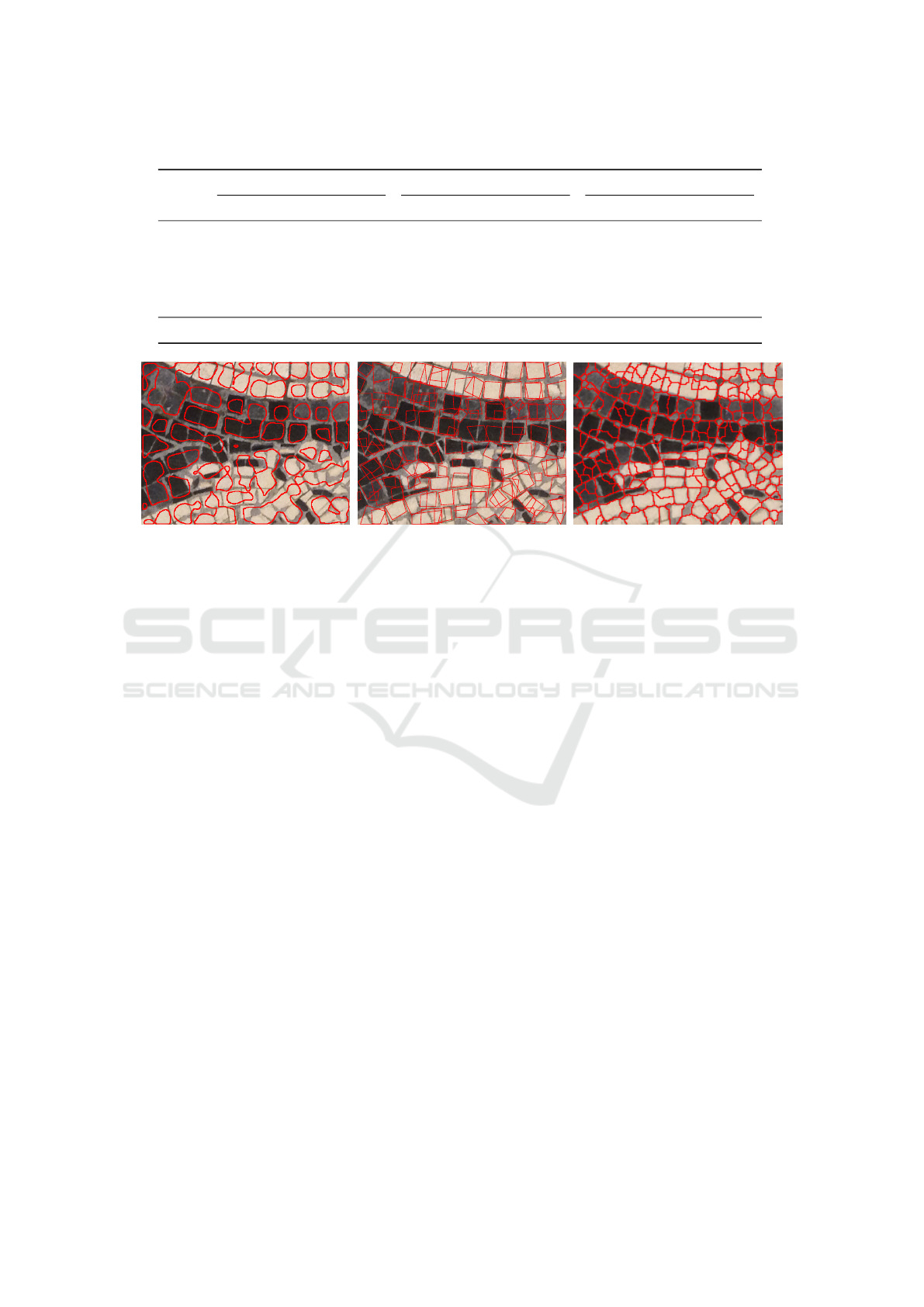
Table 2: Results obtained with our method and with GA and TOS for a subset of the dataset.
U-net with w = 0.5 GA TOS
Im. # Cnt Prec Rec Fm Cnt Prec Rec Fm Cnt Prec Rec Fm
7 0.30 0.67 0.80 0.73 0.03 0.50 0.76 0.60 0.14 0.64 0.87 0.74
8 0.28 0.59 0.71 0.64 0.03 0.42 0.63 0.50 0.54 0.56 0.72 0.63
9 0.21 0.62 0.73 0.67 0.01 0.41 0.66 0.51 0.03 0.53 0.82 0.64
10 0.52 0.65 0.70 0.67 0.07 0.50 0.63 0.56 0.06 0.49 0.68 0.57
11 0.29 0.65 0.72 0.69 0.03 0.46 0.67 0.55 0.90 0.63 0.78 0.70
Avg. 0.32 0.64 0.73 0.68 0.03 0.46 0.67 0.54 0.33 0.57 0.77 0.66
(a) U-net (b) GA (c) TOS
Figure 2: Example of segmentation of image 11 overlapped on the original image with the three methods.
5 CONCLUSIONS AND FUTURE
WORK
We considered the problem of the segmentation of
mosaic images and proposed a method based on deep
learning, namely U-net. We experimentally evaluated
our proposal on a set of 11 images of real mosaics
acquired in different conditions, with different image
quality, and with different building properties. The re-
sults suggest that our method is effective, scoring the
better value for the most relevant index on the major-
ity of images used in the comparison.
We think that our results constitute a further ev-
idence that modern deep learning systems can help
solving tasks in a variety of fields, here in digital hu-
manities.
We believe that further improvements in mosaic
image segmentation might be obtained. The most
promising way to achieve them might be merging to-
gether two radically different techniques: the one pre-
sented in the present paper, based on deep learning,
and the one designed by Bartoli et al. (2016), based
on a different form of optimization which includes,
in the solution presentation, some domain knowledge
concerning the shape of the tiles.
ACKNOWLEDGMENTS
The experimental evaluation of this work has been
done on Amazon AWS within the “AWS Cloud Cred-
its for Research” program.
REFERENCES
Assael, Y., Sommerschield, T., and Prag, J. (2019). Restor-
ing ancient text using deep learning: a case study on
greek epigraphy. arXiv preprint arXiv:1910.06262.
Bartoli, A., Fenu, G., Medvet, E., Pellegrino, F. A., and
Timeus, N. (2016). Segmentation of mosaic im-
ages based on deformable models using genetic al-
gorithms. In International Conference on Smart Ob-
jects and Technologies for Social Good, pages 233–
242. Springer, Springer.
Benyoussef, L. and Derrode, S. (2011). Analysis of an-
cient mosaic images for dedicated applications. In
Stanco, F., Battiato, S., and Gallo, G., editors, Digital
Imaging for Cultural Heritage Preservation: Analy-
sis, Restoration, and Reconstruction of Ancient Art-
works. CRC Press.
C¸ ic¸ek,
¨
O., Abdulkadir, A., Lienkamp, S. S., Brox, T., and
Ronneberger, O. (2016). 3d u-net: learning dense vol-
umetric segmentation from sparse annotation. In In-
ternational conference on medical image computing
and computer-assisted intervention, pages 424–432.
Springer.
Mosaic Images Segmentation using U-net
491

Comes, R., Buna, Z., and Badiu, I. (2014). Creation and
preservation of digital cultural heritage. Journal of
Ancient History and Archaeology, 1(2).
Falk, T., Mai, D., Bensch, R., C¸ ic¸ek,
¨
O., Abdulkadir, A.,
Marrakchi, Y., B
¨
ohm, A., Deubner, J., J
¨
ackel, Z., Sei-
wald, K., et al. (2019). U-net: deep learning for cell
counting, detection, and morphometry. Nature meth-
ods, 16(1):67.
Fazio, L., Brutto, M. L., and Dardanelli, G. (2019). Sur-
vey and virtual reconstruction of ancient roman floors
in an archaeological context. International Archives
of the Photogrammetry, Remote Sensing and Spatial
Information Sciences, 42(2/W11).
Fenu, G., Jain, N., Medvet, E., Pellegrino, F. A., and Pi-
lutti Namer, M. (2015). On the assessment of seg-
mentation methods for images of mosaics. In In-
ternational Conference on Computer Vision Theory
and Applications-VISAPP, volume 3, pages 130–137.
SciTePress, SciTePress.
Kingma, D. P. and Ba, J. L. (2015). Adam: A method for
stochastic optimization. In Proceedings of the 3rd In-
ternational Conference on Learning Representations
(ICLR).
Kohl, S., Romera-Paredes, B., Meyer, C., De Fauw, J., Led-
sam, J. R., Maier-Hein, K., Eslami, S. A., Rezende,
D. J., and Ronneberger, O. (2018). A probabilis-
tic u-net for segmentation of ambiguous images. In
Advances in Neural Information Processing Systems,
pages 6965–6975.
Monti, M. and Maino, G. (2011). Image processing and
a virtual restoration hypothesis for mosaics and their
cartoons. In International Conference on Image Anal-
ysis and Processing, pages 486–495. Springer.
Neum
¨
uller, M., Reichinger, A., Rist, F., and Kern, C.
(2014). 3d printing for cultural heritage: Preserva-
tion, accessibility, research and education. In 3D Re-
search Challenges in Cultural Heritage, pages 119–
134. Springer.
Ronneberger, O., Fischer, P., and Brox, T. (2015). U-net:
Convolutional networks for biomedical image seg-
mentation. In International Conference on Medical
image computing and computer-assisted intervention,
pages 234–241. Springer.
Vincent, L. and Soille, P. (1991). Watersheds in digital
spaces: an efficient algorithm based on immersion
simulations. IEEE Transactions on Pattern Analysis
and Machine Intelligence, 13(6):583–598.
Youssef, L. B. and Derrode, S. (2008). Tessella-oriented
segmentation and guidelines estimation of ancient
mosaic images. Journal of Electronic Imaging,
17(4):043014.
Zhang, Z., Liu, Q., and Wang, Y. (2018). Road extraction
by deep residual u-net. IEEE Geoscience and Remote
Sensing Letters, 15(5):749–753.
ICPRAM 2020 - 9th International Conference on Pattern Recognition Applications and Methods
492
