Prediction of Dynamical Properties of Biochemical Pathways
with Graph Neural Networks
Pasquale Bove, Alessio Micheli, Paolo Milazzo and Marco Podda
Department of Computer Science, University of Pisa, Largo B. Pontecorvo, 3, 56127, Pisa, Italy
Keywords:
Systems Biology, Pathway Modelling, Robustness, Deep Learning, Graph Neural Networks.
Abstract:
Biochemical pathways are often represented as graphs, in which nodes and edges give a qualitative descrip-
tion of the modeled reactions, while node and edge labels provide quantitative details such as kinetic and
stoichiometric parameters. Dynamical properties of biochemical pathways are usually assessed by performing
numerical (ODE-based) or stochastic simulations in which quantitative parameters are essential. These sim-
ulation methods are often computationally very expensive, in particular when property assessment requires
varying parameters such as initial concentrations of molecules. In this paper we propose the use of a Deep
Neural Network (DNN) to predict such dynamical properties relying only on the graph structure. In partic-
ular, our model is based on Graph Neural Networks. We focus on the dynamical property of concentration
robustness, which is the ability of the pathway to maintain the concentration of some molecules within certain
intervals despite of perturbation in the initial concentration of other molecules. The use of DNNs can allow
robustness to be predicted by avoiding the burden of performing a huge number of numerical or stochastic sim-
ulations. Moreover, once trained, the model could be applied to predicting robustness properties for pathways
in which quantitative parameters are not available.
1 INTRODUCTION
In order to understand the mechanisms underlying the
functioning of living cells, it is necessary to analyze
their activities at the biochemical level. Biochem-
ical pathways (or networks) are complex dynami-
cal systems in which molecules interact with each
other through chemical reactions. In these reactions,
molecules can take different roles: reactant, product,
promoter and inhibitor.
Chemical kinetics laws, such as the law of mass
action, allow describing and analysing the dynam-
ics of a set of chemical reactions through Ordinary
Differential Equations (ODEs). Moreover, stochastic
modelling and simulation approaches, typically based
on one of the many variants of Gillespie’s simula-
tion algorithm (Gillespie, 1977) are often adopted in
the case of pathways involving molecules available in
small concentrations, which make the dynamics of re-
actions sensitive to random events.
Biochemical pathways are very often represented
as graphs. Many different graphical notations exist
(see, e.g., Karp and Paley (1994); Reddy et al. (1993);
Le Novere et al. (2009)). Most of them essentially
represent molecules as nodes and reactions as multi-
edges or as additional nodes. Graphical notations are
very common since they provide a quite natural visual
representation of the involved reactions. These nota-
tions enable network and structural analysis methods
to be applied to the investigation of properties of the
pathway as a whole. Moreover, they can usually be
translated into ODEs or stochastic models in order to
apply standard numerical simulation techniques.
Models of biochemical pathways are typically
used to investigate dynamical properties of these sys-
tems such as the reachability of steady states, the
occurrence of oscillatory behaviors, causalities be-
tween species, and robustness. The assessment of
these properties often requires the execution of sev-
eral numerical or stochastic simulations. In particu-
lar, robustness (Kitano, 2004), i.e. the maintenance
of some concentration levels against the perturbation
of parameters or initial conditions, is a key property
of many biochemical pathways. Its assessment usu-
ally requires a huge number of simulations in order to
extensively explore the parameter space.
This paper aims at investigating the applicabil-
ity of Machine Learning (ML), and in particular
Deep Learning (Goodfellow et al., 2016) methods for
graphs to the prediction of dynamical properties of
32
Bove, P., Micheli, A., Milazzo, P. and Podda, M.
Prediction of Dynamical Properties of Biochemical Pathways with Graph Neural Networks.
DOI: 10.5220/0008964700320043
In Proceedings of the 13th International Joint Conference on Biomedical Engineering Systems and Technologies (BIOSTEC 2020) - Volume 3: BIOINFORMATICS, pages 32-43
ISBN: 978-989-758-398-8; ISSN: 2184-4305
Copyright
c
 2022 by SCITEPRESS – Science and Technology Publications, Lda. All r ights reserved

biochemical pathways. The assumption at the basis of
this study is that some dynamical properties of path-
ways could be correlated with topological properties
of the graphs modeling such pathways. The idea is
then to use ML methods to automatically infer those
topological properties in a dataset of pathway graphs,
and predict the dynamical property of interest on their
basis. Labels in the dataset are determined by per-
forming numerical simulations based on ODE models
of the associated pathways. If the initial assumption
is correct, the obtained ML model could be able to
predict whether the studied dynamical property holds,
thus reducing the need of performing expensive nu-
merical or stochastic simulations. Moreover, once
trained the ML model could be applied to predicting
dynamical properties of pathways for which quantita-
tive parameters are not available. To our knowledge,
this is the first work that addresses this open chal-
lenge, in contrast with many approaches in literature
that mainly focus on inferring the parameters of a sin-
gle pathway or the relationships between its species.
In summary, we test the strong assumption that net-
work structure alone is sufficient to predict dynamical
properties of pathways, and verify experimentally to
which extent it is.
In this study, we focus on the assessment of the
dynamical property of robustness (Kitano, 2004) on
the basis of a graph representation of biochemical
pathways in terms of Petri nets (Reddy et al., 1993).
We start from the creation of a dataset of Petri nets
obtained from curated pathway models in SBML for-
mat downloaded from the BioModels
1
database (Li
et al., 2010). Robustness indicators of these pathways
(to be used as labels in the dataset) have been com-
puted by performing ODE-based simulations using
the libRoadRunner Python library (Somogyi et al.,
2015), which exploits GPU computing power. In par-
ticular, given a pathway model and a pair of molecu-
lar species (called input and output species), the com-
puted robustness value measures how much the con-
centration of the output species at the steady state is
influenced by perturbations of the initial concentra-
tion of the input species. This is a notion of concen-
tration robustness (Shinar and Feinberg, 2010) which
is to some extent correlated with the notion of global
sensitivity (Zi, 2011). To predict the robustness indi-
cators associated to pairs of input/output species of a
given pathway, we propose the following framework:
first, we construct a subgraph of the pathway, which
contains the input and output node as well as all the
nodes that influence the reaction dynamics. Then, we
develop a Deep Neural Network (DNN) model com-
posed of two modules trained jointly: a Graph Neu-
1
BioModels: https://www.ebi.ac.uk/biomodels/
ral Network (GNN) (Scarselli et al., 2009; Micheli,
2009) that processes the subgraph, automatically ex-
tracting structural information that correlate with its
robustness in the form of a vector; and a Multi-Layer
Perceptron (Murtagh, 1991) predictor which, given
the vectorial representation inferred by the GNN,
classifies the graph as robust or not. We assess the
performances of this model on out-of-sample (unseen
during training) data, showing that we are indeed able
to predict robustness with reasonable accuracy. The
rest of the paper is structured as follows. Section 2
contains some background notions of robustness and
Petri nets modeling of pathways. In Section 3 we de-
scribe our methodology, defining the predictive task
as well as providing details of the Deep Neural Net-
work model. Section 4 describes the experimental
setup. In Section 5 we discuss the results of our exper-
iments. Finally, in Section 6 we draw our conclusions
and discuss future work.
2 BACKGROUND
2.1 Biological Robustness
Robustness is a property observed in many biologi-
cal systems. It is the ability of the system to maintain
its functionalities again external and internal perturba-
tions (Kitano, 2004). A general formalization of the
notion of robustness has been proposed in (Kitano,
2007), where the robustness R of a system s with re-
gard to a specific functionality a and against a set of
perturbations P is defined as:
R
s
a,P
=
Z
P
ψ(p)D
s
a
(p)d p
In this definition, ψ(p) is the probability for per-
turbation p to take place, and D
a
(p) is a relative
evaluation function for functionality a under pertur-
bation p. Let the viability of a functionality to be
a measure of the ability of the cell to carry out it.
This could be expressed, for instance, in terms of
the synthesis/degradation rate or concentration level
of some target substance, in terms of cell growth rate,
or in terms of any other suitable quantitative indicator.
Function D
a
(p) gives the viability of a under pertur-
bation p relative to the viability of the same function-
ality in normal conditions. By assuming that in the
absence of perturbations functionality a is carried out
in an optimal way, we have D
a
(p) = 0 for perturba-
tions causing the system to fail in a, D
a
(p) = 1 in the
cases of no or irrelevant perturbations (i.e. having no
influence), and 0 < D
a
(p) < 1 in the case of relevant
perturbations.
Prediction of Dynamical Properties of Biochemical Pathways with Graph Neural Networks
33

Kitano’s formulation of robustness has been im-
proved in (Rizk et al., 2009), where functionalities to
be maintained are described as linear temporal logic
(LTL) formulas and the impact of perturbations is
measured through a notion of violation degree mea-
suring the distance between the dynamics of the per-
turbed system and the LTL formula. Many more spe-
cific definitions exist, which differ either in the class
of biological systems they apply to, or in the way the
functionality to be maintained is expressed (Larhlimi
et al., 2011). In the case of biochemical pathways, ro-
bustness can be expressed in terms of maintenance of
the concentration of some species in the steady state
against perturbations in the kinetic parameters or in
the initial concentration of some other species. This is
formally expressed by the notion of absolute concen-
tration robustness proposed in (Shinar and Feinberg,
2010).
A generalization of absolute concentration robust-
ness, called α-robustness, has been proposed in (Nasti
et al., 2018), where concentration intervals are consid-
ered both for the perturbed molecules (input species)
and for the molecules whose concentration is main-
tained (output species). Roughly speaking, a bio-
chemical pathway is α-robust with respect to a given
set of initial concentration intervals if the concentra-
tion of a chosen output molecule at the steady state
varies within an interval of values [k − α/2,k + α/2]
for some k ∈ R. A relative version of α-robustness can
be obtained simply by dividing α by k. The notion of
α-robustness is related with the notion of global sensi-
tivity (Zi, 2011) which typically measures the average
effect of a set of perturbations.
Assessment of robustness properties is usually ob-
tained by performing exhaustive (in the parameter
space) numerical simulations (Rizk et al., 2009; Iooss
and Lema
ˆ
ıtre, 2015). In some particular cases there
exist sufficient conditions on the biological network
structure that can avoid simulations to be performed
(Shinar and Feinberg, 2010). Moreover, the assess-
ment of monotonicity properties in the dynamics of
the network may allow the number of simulations to
be significantly reduced (Gori. et al., 2019).
2.2 Petri Nets Modeling of Pathways
Biochemical pathways are essentially sets of chemi-
cal reactions. A chemical reaction can be described
by a multiset of reactants, a multiset of products, and
the kinetic constant of the reaction. Reactants and
products are multisets since more than one instance
of the same molecule could be consumed or produced
by a reaction. Moreover, according to the standard
chemical law of mass action, the rate of occurrence
of the reaction is given by its kinetic constant multi-
plied by the concentrations of its reactants in consid-
ered chemical solution. For example, let us assume A
and B to be molecules and let us use the same symbols
A and B to denote the respective concentrations in ki-
netic formulas. We have that A + B
k
−→ 2B describes
the chemical reaction in which reactants A and B are
transformed into two instances of B (the products) at a
rate given by the kinetic formula kAB (as is happens,
for example, in Lotka-Volterra reactions).
In the context of biochemistry (and of biochemi-
cal pathways) reactions are described at a higher level
of abstraction, by allowing the modeler to include in
their description molecules that act either as promoter
or as inhibitor. This means that there are additional
molecules associated with reactions, that are not listed
among reactants and products, but which may have a
role in the kinetic formula (that now could no longer
follow the mass action principle).
For example, in the SBML language (Hucka et al.,
2018), a standard XML-based modeling language for
biochemical pathways, each reaction can be associ-
ated with a number of modifiers the concentration of
which can be used in the kinetic formula of the reac-
tion. In Figure 1a we show a table describing a bio-
chemical pathway as a set of reactions (first column).
Each reaction is associated with its kinetic formula
(third column). Moreover, a couple of reactions are
associated with a modifier (second column), namely
A and F. From the kinetic formulas of those two re-
actions it is clear that A acts as a promoter of reaction
C + D → E (the rate is proportional to the concen-
tration of A) and that F acts as inhibitor of reaction
G → H (the rate is inversely proportional to the con-
centration of F). Kinetic formulas can then be used to
construct a system of Ordinary Differential Equations
(ODEs) as shown in Figure 1b.
A graphical representation of biochemical path-
ways can be given in terms of Petri nets (Reddy et al.,
1993; Gilbert et al., 2007). Petri nets have been orig-
inally proposed as a formalism of the description and
analysis of concurrent systems (Peterson, 1977), but
later have been adopted for the modeling of other
kinds of systems, such as biological ones. Several
variants of Petri nets exist. For the aim of this work
we consider a version of continuous Petri nets (Gilbert
et al., 2007) with promotion and inhibition arcs and
general kinetic functions. We call this variant path-
way Petri nets.
A pathway Petri net is essentially a bipartite graph
with different types of arcs and with labels in both
edges and arcs. According to standard Petri nets ter-
minology, the two types of edges are called places and
transitions. The dynamics (or semantics) of a Petri
BIOINFORMATICS 2020 - 11th International Conference on Bioinformatics Models, Methods and Algorithms
34

Reaction Mod Kinetics
A + B → 2B k
1
AB
B → A k
2
B
C + D → E A k
3
CDA
E → F k
4
E
F → E k
5
F
G → H F
k
6
G
1+2F
H → G k
7
G
(a) Reactions
dA
dt
= −k
1
AB + k
2
B
dB
dt
= k
1
AB − k
2
B
dC
dt
= −k
3
CDA
dD
dt
= −k
3
CDA
dE
dt
= k
3
CDA − k
4
E + k
5
F
dF
dt
= k
4
E − k
5
F
dG
dt
= −
k
6
G
1+2F
+ k
7
G
dH
dt
=
k
6
G
1+2F
− k
7
G
(b) ODEs
(c) Pathway Petri net
Figure 1: Example of biochemical pathway: list of reactions with information on modifiers and kinetic formulas (as they can
be obtained from a SBML model), corresponding ODE model and pathway Petri net.
net in a continuous setting is described by a system of
ODEs with one equation for each place. In the case
of pathways, such a system of ODEs corresponds ex-
actly to the one that can be obtained from the modeled
chemical reactions (as in Figure 1b). A state of a path-
way Petri net (called marking) is then an assignment
of positive real values to the variables of the ODEs.
We denote with M the set of all possible markings.
A pathway Petri net can be formally defined as a
tuple N = (P, T, f , p, h,v,m
0
) where:
• P and T are finite, non empty, disjoint sets of
places and transitions, respectively;
• f : ((P × T ) ∪ (T × P)) → N
≥0
defines the set of
directed arcs, weighted by non-negative integer
values;
• p,h ⊆ (P × T ) are the sets of promotion and inhi-
bition arcs;
• v : T → Ψ, with Ψ = M → R
≥0
, is a function that
assigns to each transition a function correspond-
ing to the computation of a kinetic formula to ev-
ery possible marking m ∈ M;
• m
0
∈ M is the initial marking.
The visual representation of a pathway Petri net is
shown in Figure 1c, that is the net corresponding to
the pathway in Figure 1a. Places P and transitions
T of a pathway Petri net represent molecules and re-
actants, and are depicted as circles and rectangles,
respectively. In the figure, places contain the name
of the corresponding molecule. Directed arcs f , de-
picted as standard arrows, connect reactants to reac-
tions and reactions to products. The weight of such
arcs (omitted if 1) correspond to the multiplicity (i.e.
stoichiometry) of the connected molecules as reac-
tant/product of the reaction. If 0 the whole arc is omit-
ted. Promotion and inhibition arcs, p and h, connect
molecules to the reactions they promote or inhibit, re-
spectively, and they are depicted as arrows ended by a
filled dot or a T. The kinetic formulas (actually, only
the constants k
i
, for the sake of readability) described
by the labeling function v are shown inside the rect-
angles of the corresponding transitions. We assume
molecules connected through promotion arcs to give
a positive contribution to the value of the kinetic for-
mula, while molecules connected through inhibition
arcs to give a negative (inversely proportional) contri-
bution. Finally, the initial marking m
0
is not depicted
in the figure: it has to be described separately.
3 METHODS
3.1 Graph Preprocessing
Pathway Petri nets representations of biochemical
pathways are the basis for the creation of a dataset
of graphs, which will be the input of our DNN model.
We made some critical choices about the information
in the Petri nets to be preserved in our dataset. In par-
ticular, in order to let the ML method focus on the
topological properties of the graphs, we decided to
omit the following information from the Petri nets:
• Kinetic formulas;
• Multiplicities of reactants and products (i.e. arc
labels);
• The initial marking m
0
.
Consequently, by considering again the biochemical
pathway presented in Figure 1 we have that, by re-
moving the mentioned information from its Petri net,
we obtain the result shown in Figure 2.
In order to be used by the DNN model, we re-
formulate the “cleaned” Petri nets models of path-
ways into standard graphs. Hence, we represent a bio-
chemical pathway as a directed graph G = hV
G
,E
G
i,
where V
G
= {v
1
,v
2
,...,v
n
} is a set of nodes, and
Prediction of Dynamical Properties of Biochemical Pathways with Graph Neural Networks
35

Figure 2: Pathway Petri net in which kinetic formulas and
arc labels have been omitted.
E
G
= {hu, vi | u,v ∈ V } is a set of edges. Furthermore,
we define the neighborhood function of a node v as
N (u) = {v | (u,v) ∈ E
G
} for each node u ∈V
G
. Nodes
can be of two types: molecules, denoted V
G
mol
, and
reactions, denoted V
G
react
, with V
G
= V
G
mol
∪V
G
react
and
V
G
mol
∩V
G
react
=
/
0. Edges can be of three types: stan-
dard, denoted E
G
std
, promoters, denoted E
G
pro
, and in-
hibitors, denoted E
G
inh
. Again, E
G
= E
G
std
∪ E
G
pro
∪ E
G
inh
and E
G
std
∩ E
G
pro
∩ E
G
inh
=
/
0.
Given a pathway Petri net N = (P,T, f , p,h, v,m
0
)
the corresponding graph G can be obtained by set-
ting V
G
mol
= P, V
G
react
= T, E
G
std
= {hu,vi ∈ (P × T ) ∪
(T × P) | f (hu,vi) > 0}, E
G
pro
= p, E
G
inh
= h. By con-
struction, the obtained graph turns out to be bipartite.
For graphs obtained in this way we adopt the same
visual representation that we introduced for pathway
Petri nets without kinetic formulas and arc multiplic-
ities (see Figure 2).
Let us define G
0
, an enriched version of G, as fol-
lows: initially, V
G
0
= V
G
, E
G
0
= E
G
. Then, if hu,vi ∈
E
G
std
is a standard edge connecting a molecule to a
reaction, we augment E
G
0
adding the same edge but
with reversed direction. Formally, we define E
G
0
std
=
E
G
std
∪ {hv, ui | hu, vi ∈ E
G
std
,u ∈ V
G
mol
,v ∈ V
G
react
}. Note
that we do not reverse neither standard edges from
reactions to molecules, nor promotion and inhibition
edges.
Figure 3: Enriched version of the graph in Figure 2.
(a) I = A, O = B
(b) I = C,O = F
(c) I = A, O = H
Figure 4: Examples of subgraphs of the graph in Figure 2
induced by different input/output node pairs (u,v) = (I,O).
The enriched version G
0
of the graph G obtained
from the Petri net in Figure 2 is shown in Fig-
ure 3. It now represents influence relationships be-
tween molecules and reactions. There is an edge (of
any type) from a molecule to a reaction if and only
if a perturbation in the concentration of the molecule
determines a change in the reaction rate (that should
be computed from the omitted kinetic formula). Sim-
ilarly, there is an edge from a reaction to a molecule
if and only if a perturbation in the reaction rate deter-
mines a change in the dynamics of the concentration
of that molecule. This is intuitive for edges connect-
ing reactions to products: the dynamics of the product
accumulation is determined by the reaction rate. As
regards the reversed edges we added in the enriched
graph, this is motivated by the fact that a perturba-
tion in the reaction rates determines a variation in the
consumption of the reactants. The enriched graph es-
sentially corresponds to the influence graph that could
be computed from the Jacobian matrix containing the
partial derivatives of the system of ODEs of the mod-
elled molecular pathway (Fages and Soliman, 2008).
Since we want to assess a property, concentration
robustness, which expresses a relationship between
an input and an output molecules of a given path-
way, we can, through the enriched graph G
0
, deter-
mine which portion of the graph modelling the path-
way is relevant for the assessment of the property.
Given a graph G, and a pair of nodes u and v, we
define S
uv
= hV
S
uv
,E
S
uv
i, the subgraph of G induced
by the input/output node pair (u,v), informally as fol-
lows: S
uv
is the smallest subgraph of G whose node
set contains u, v, as well as nodes in every possible
oriented path from u to v in G
0
. We remark that S
uv
is
a subgraph of G, although it is computed on the basis
BIOINFORMATICS 2020 - 11th International Conference on Bioinformatics Models, Methods and Algorithms
36

of the paths in G
0
. Figure 4 shows some examples of
induced subgraphs extracted from the graph in Fig-
ure 2. Induced subgraphs will allow us to apply the
ML approach only on the portions of the graph which
are relevant for the property by getting rid of unnec-
essary nodes and edges.
3.2 Graph Neural Networks
Traditional ML modeling assumes that the input data
is represented as fixed-size, continuous vectors. In
contrast, graphs are discrete objects by nature, whose
size is variable. Hence, learning from graphs is
not straightforward; to be exploited by ML mod-
els, graph structure, as well as information contained
in nodes and edges, must be mapped jointly into a
shared, real-valued vector. Of course, the effective-
ness of the mapping is closely related to how much
the original relationships are preserved: for example,
distances between graphs in graph space should re-
main relatively consistent between vectors in the map-
ping space. GNNs are neural networks that are able
to learn meaningful graph-to-vector mappings adap-
tively from data. The core idea of GNNs is to as-
sociate a state vector, also called embedding, to each
node of a graph; initially, the embedding is a vector
of node descriptors. Then, the embedding of each
node is updated as a function of the embeddings of
its neighboring nodes. We refer to this transformation
as applying a GNN layer
2
to the node. This process
can be iterated multiple times, by composing (“stack-
ing”) these layer transformations. Taking Figure 5 as
a visual example, we now describe how GNNs work.
Let us assume that our reference graph is composed of
the node to be processed, v, and its neighboring nodes
(shaded in the figure) u
1
, u
2
, and u
3
. Suppose that we
have already applied i GNN layers to the node, and
i + 1 GNN layers to its neighboring nodes. The task
is to update the embedding of the current node, h
i
v
,
through the application of the i + 1 GNN layer; this
initial situation is shown in Figure 5a. The first oper-
ation performed by a GNN layer is neighborhood ag-
gregation, shown in Figure 5b. Specifically, a neigh-
boring function N (v) selects nodes (or a subset of
nodes) in the neighborhood of v, and combines their
embedding through a permutation-invariant
3
function
Γ, producing the neighborhood vector h
i+1
N (v)
. The
subsequent phase is shown in Figure 5c, in which the
2
In accordance to the terminology of DNNs, where lay-
ers are functions that apply a data-driven transformation to
their inputs (Goodfellow et al., 2016).
3
A function f is invariant with respect to a permutation
π iff f (x) = f (π(x)); in our case, the input x are sets of node
embeddings.
neighborhood vector and the current node embedding
h
i
v
(shown shaded in the figure) are combined together
by a function Φ to obtain the updated node embed-
ding. In its entirety, the node embedding h
i+1
v
is com-
puted as follows:
h
i+1
v
= σ(w
i
· Φ(h
i
v
,h
i+1
N (v)
)),
where σ is a non-linear function called activation, and
w is a vector of “trainable” weights, whose values
are tuned (usually with gradient descent) to best ap-
proximate the relationship between the input graph
and the target property. Notice that each new layer
reuses the embedding computed at the previous layer
as its input; also, recall that the initial embedding h
0
v
is a vector of node descriptors (features). As the num-
ber of layers increases, node embeddings incorporate
(through the neighborhood vector) information com-
ing from nodes farther away: in particular, in the i-th
layer, nodes receive information by nodes up to i hops
from them (where a hop is defined as the shortest un-
weighted path between two nodes).
Once a layer is applied simultaneously to all the nodes
in the graph (which corresponds to visiting each node
in the graph in any order), one can produce a single
embedding for the entire graph by performing node
aggregation: that is, compute a single embedding rep-
resenting the entire graph as a function of the embed-
dings of the graph nodes. Specifically, one can com-
pute H
i
G
, the graph embedding associated to the i-th
GNN layer, by performing:
H
i
G
= τ({h
i
v
| v ∈ V
G
}),
where τ is another permutation-invariant function
called readout. Ultimately, after stacking L GNN lay-
ers, one obtains L different graph embeddings, each
one constructed using information coming from a pro-
gressively “broader” view of the graph. At this point,
the common practice is to concatenate all these em-
beddings into a single vector and obtain H
G
, a final
graph embedding which can be used as input by com-
mon ML algorithms for tasks such as regression or
classification. Note that different choices of Γ, Φ and
τ result in different GNN variants. For example, Γ
and τ can be vector sum, and Φ can be simple vec-
tor concatenation, or a more complicated function ap-
proximated by a neural network. Details specific to
our implementation are discussed in Section 4.2.
3.3 Model
Here, we describe our learning framework in de-
tail. We are given a set of pathway Petri networks
G = {G
1
,G
2
,... ,G
N
}, represented as graphs follow-
ing the formulation in Section 3.1. Each graph is asso-
ciated with a set of tuples T
G
: {(S
uv
, r) | u,v ∈ V
G
, r ∈
Prediction of Dynamical Properties of Biochemical Pathways with Graph Neural Networks
37

(a) Initial graph (b) Neighbor aggregation
(c) Embedding update (weight multiplica-
tion and non-linearity not shown).
Figure 5: An example of GNN processing at the node level.
[0,1] ⊆ R}, where u and v are graph nodes, S
uv
is their
induced subgraph, and r expresses how much the out-
put node v is robust to perturbations to the input node
v. Note that our task is to learn to predict whether the
induced subgraph associated to a pair of input/output
nodes is robust or not, as opposed to learn the exact
value of the property. Hence, in ML terms, we tackle
a classification problem where our graph labels be-
long to the discrete set {0,1}, with 0 indicating not
robust, and 1 indicating robust. It is straightforward
to transition from the original problem to a classifica-
tion one by simply discretizing robustness values into
indicators as follows:
t =
(
1 if r > 0.5
0 otherwise.
Our reference set thus becomes: T
G
: {(S
uv
, t) |
u,v ∈ V
G
mol
, t ∈ {0,1}}. As additional notation, we
will refer to 1 as the ”positive class”, and 0 as the
”negative class”. Having collected all the neces-
sary information, we build a dataset of induced sub-
graphs and their associated robustness indicators D =
S
G∈G
{T
G
}. With this premise, our predictive task
is the following: given a previously unseen path-
way network and a pair of input/output species nodes,
we seek to predict the associated robustness indicator
with reasonable accuracy. In our graph framework,
this corresponds to learn a function f (S
uv
) =
ˆ
t that
given an induced graph S
uv
over nodes u and v, pre-
dicts a robustness value
ˆ
t which is as close as possible
to the ground truth t, i.e. we wish to minimize the fol-
lowing binary cross-entropy (Janocha and Czarnecki,
2017) (BCE) objective function:
BCE(D) = −
1
M
∑
T
G
∈D
∑
S,t∈T
G
t log(
ˆ
t) + (1 −t) log(1 −
ˆ
t),
with M = |D| · |T
G
|, where we drop the subscript
notation on S for ease of notation. We propose to ap-
proximate f using a DNN composed of a GNN that
receives as input an induced subgraph S (defined over
a certain input/output node pair (u,v)), and produces
as output an embedding H
S
. This embedding is taken
as input by an MLP classifier, which outputs a value
between 0 and 1. The DNN output can be interpreted
as the probability of v being robust to perturbations
in u, given the structural information of the induced
subgraph. The corresponding predicted indicator can
be obtained by simply rounding this probability to the
nearest integer. More formally, we estimate the un-
known function f with the following:
f (S) ≈ MLP
φ
(H
S
),
where H
S
is the induced subgraph embedding ob-
tained by the GNN in a similar fashion as described
in Section 3.2, and φ are weights that are learned us-
ing gradient descent. Figure 6 shows a high-level
overview of our model.
4 EXPERIMENTS
4.1 Dataset Construction
Our dataset originates from 706 SBML models of bio-
chemical pathways downloaded from the BioModels
database (Le Novere et al., 2006). They correspond to
the complete set of manually curated models present
in the database at the time we started the construction
of the dataset
4
. From these models, we built the as-
sociated Petri nets representations, which were saved
as graphs in DOT format
5
. For the translation of the
SMBL models into (pathway) Petri nets we developed
a Python script that, for each reaction in the SMBL
4
May 2019.
5
The DOT graph description language specification,
available at: https://graphviz.gitlab.io/ pages/doc/info/lang.
html
BIOINFORMATICS 2020 - 11th International Conference on Bioinformatics Models, Methods and Algorithms
38

Figure 6: A high-level overview of our model to predict robustness (using three GNN layers for ease of visualization). The
big black arrow connecting layers indicates that node states computed at layer i are used to initialize layer i + 1. Note how
each layer computes a different graph embedding (where color intensity is used as a proxy for value magnitude).
model extracts reactants, products and modifiers. It
also checks the kinetic formula in order to determine
whether each modifier is either promoter or an in-
hibitor. Subsequently, empty graphs (not containing
any node) and duplicates were discarded. The remain-
ing ones were translated into graphs compliant with
the notation described in Section 3.1, and the cor-
responding induced subgraphs for each input/output
combination were extracted. At this point, in order to
have a size-homogeneous dataset of graphs and since
we did not have any previous knowledge of the effec-
tiveness of GNNs on this task, we focused on induced
subgraphs with at most 40 nodes. We plan to extend
our results to larger graphs in future works. After this
preprocessing, we ended up with a dataset of 7013 in-
duced subgraphs.
The robustness values to be used as labels of the
induced subgraphs have been computed by follow-
ing the relative α-robustness approach. The dynam-
ics of each biochemical pathway has been simulated
by applying a numerical solver (the libRoadRunner
Python library) to its ODEs representation. Ref-
erence initial concentrations of involved molecules
have been obtained from the original SBML model
of each pathway. Moreover, 100 simulations have
been performed for each molecule of the pathway
by perturbing its initial concentration in the range
[−20%,+20%]. The termination of each simulation
has been set to the achievement of the steady state,
with a timeout of 250 simulated time units.
6
For each
couple of input/output molecules, we computed the
width α of the range of concentrations reached by the
output molecules by varying the input (α-robustness).
6
The concentration values obtained at the end of the sim-
ulation are considered as steady state values also in the cases
in which the timeout has been reached.
A relative robustness α has then been obtained by di-
viding α by the concentration reached by the output
when the initial concentration of the input is the refer-
ence one (no perturbation). Finally, a robustness value
r ∈ [0,1] to be used in the dataset has been computed
by comparing α (a relative representation of the out-
put range) with 0.4 (a relative representation of the
initial input range, that is 40%). Formally:
r = 1 − min(1,
α
0.4
)
4.2 Model Implementation Details
We set up the initial node embeddings as a binary
feature vector of size 3. The first position encodes
whether the corresponding node is a molecule species
(with value 1), or a reaction (with value 0). The
second position encodes whether the node is an in-
put species (with value 1) or not. The third position
encodes whether the node is an output species (with
value 1) or not. As regards the GNN, we follow the
seminal approach in (Kipf and Welling, 2017), which
uses element-wise mean as Γ, and vector sum as Φ.
Since edges can be of different types (three in our
case), we implemented the following variant of the
general GNN formulation:
h
i+1
v
= σ(
∑
k∈K
w
i
k
· Φ(h
i
v
, h
i
N (v,k)
)),
where N (v,k) is an edge-aware neighborhood func-
tion that selects only neighboring nodes of v con-
nected by an edge of type k, with K as the set of possi-
ble edge types. In other words, neighborhood aggre-
gation is repeated once for each edge type; the cor-
responding results are multiplied by a specific edge-
type weight matrix and summed together. This way,
the network can separately learn the contributions of
Prediction of Dynamical Properties of Biochemical Pathways with Graph Neural Networks
39

each different edge type. As activation function σ,
we used Rectified Linear Units (ReLU) (Glorot et al.,
2011). As regards the MLP used for the final classifi-
cation, it is composed of two linear layers followed by
ReLU non-linearities and a final linear layer that maps
its input to the output space. Moreover, intermediate
layers are regularized with Dropout (Srivastava et al.,
2014), with drop probability 0.1. In our experiments,
we optimize the number of GNN layers L, choosing in
the set {1,2, . .., 8}; the type of node aggregation (i.e.
the τ function), choosing among element-wise sum,
mean or max; and the dimension of the node state vec-
tor after the first layer, choosing between 64 and 128.
The selection of the hyper-parameters is explained in
more detail in Section 4.3. The model has been im-
plemented in Python, using the PyTorch Geometric
(Fey and Lenssen, 2019) library.
4.3 Evaluation
We evaluate the accuracy of the proposed model us-
ing 5-fold Cross-Validation (CV). In more detail, the
dataset is divided into 5 partitions of equal size. Each
partition is further split in three: the first partition
(80% of the partition size) is used as training set to
optimize the model parameters with gradient descent,
whose values are tuned according to the task and the
data at hand, as discussed in Section 3.3. Our opti-
mizer of choice is Adam (Kingma and Ba, 2015), with
a learning rate of 0.001. The second (%10 of the par-
tition size) is used as validation set to choose the opti-
mal values of the hyper-parameters, among 8 possible
number of GNN layers, 3 possible node aggregating
functions and 2 possible node embedding dimensions.
In particular, we instantiate 48 models, one for each
possible combination of the hyper-parameter values
(see Section 4.2), and record their accuracy on the
validation set; we then choose as best model the one
with the highest validation accuracy. The third (%10
of the partition size) is used as independent test set to
evaluate the best model, and compute an unbiased es-
timate of its out-of-sample accuracy. This procedure
is repeated for each partition; ultimately, it results in
5 estimates which are averaged to compute the final
test accuracy. Notice that this procedure does not use
data already ”seen” by the model, either during train-
ing or validation, to assess its performance. Impor-
tantly, we noticed a class imbalance in favour of ro-
bust graphs; in fact, approximately 73% of subgraphs
were labelled with the positive class. Hence, only dur-
ing model training, we oversampled the minority class
and trained the model with an equal number of posi-
tive and negative examples. Our experiments required
3 days of computation on a single Tesla M40 GPU.
5 RESULTS
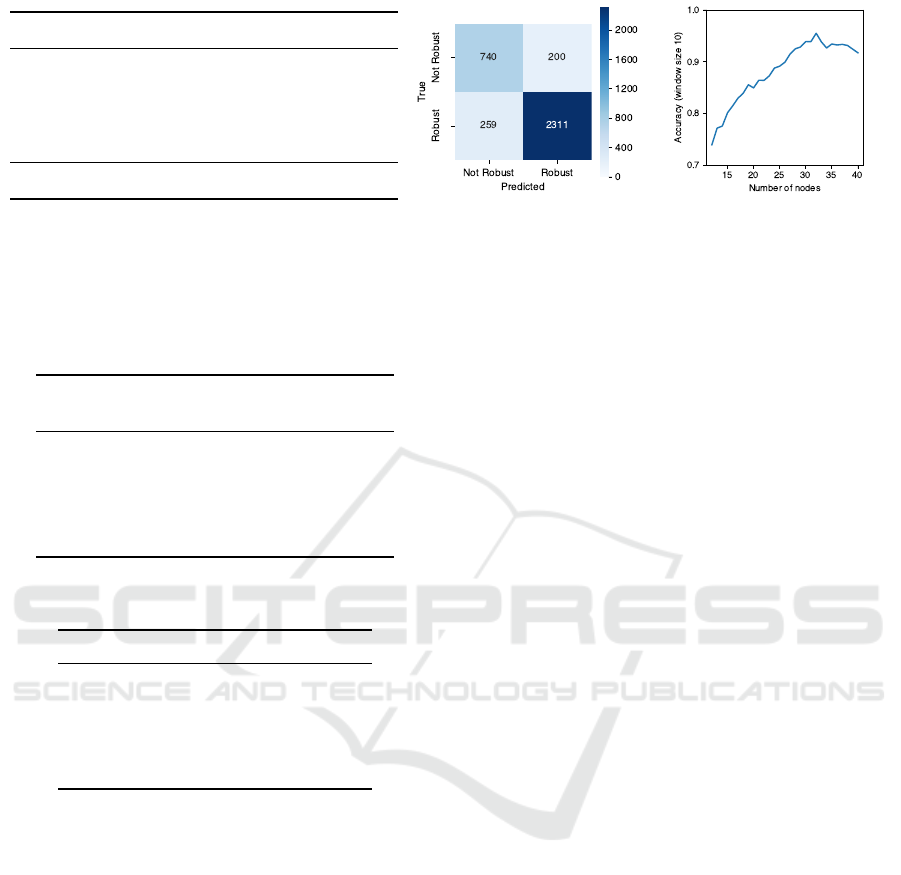
Figure 7a reports the accuracy obtained by our model,
averaged over the 5 test partitions, where the first four
rows display the accuracy stratified according to the
number of nodes of subgraphs in the test set. To show
the effectiveness of our method, we compare against
a baseline that predicts the most frequent class in the
test set, which we term the Null model. Note that,
due to label stratification, class proportions are equal
in all 5 test partitions, thus the overall accuracy of
the Null model is the same in all folds; indeed, the
associated standard deviation is 0. As can be seen,
our model consistently outperforms the baseline in all
considered strata. Figure 7b shows the confusion ma-
trix obtained by the model over the entire dataset, em-
phasizing the positive results of our model. As addi-
tional information, we report that our model obtained
an overall sensitivity of 0.7873 ± 0.0756 and an over-
all specificity of 0.8992 ± 0.0121.
The table also highlights that our model performs
better when predicting graphs with a large number
of nodes. In particular, for graphs with number of
nodes ranging from 21 to 30, the model obtains the
best predictive performance (over 93%), while for the
largest graphs (31-40 nodes), it obtains the highest
improvement with respect to the baseline (approxi-
mately 20%). This trend is shown more clearly in
Figure 7c, where we plot the improvement in accu-
racy as the number of nodes increases, using a sliding
window of size 10 to smooth the effect of outliers.
The lower prediction accuracy in the case of small
graphs (1-10 nodes) can be explained by observing
that we trained the model on a dataset of graphs in
which kinetic, stoichiometric and initial concentra-
tion parameters have been omitted. The smaller is
the graph, the higher is, in general, the influence on
its dynamics of these parameters. For example, let us
consider again the biochemical pathway introduced in
Figure 1 and the corresponding graph depicted in Fig-
ure 2. Moreover, let us consider the following kinetic
and initial concentration (marking) parameters:
k1 = 1.0 k3 = 0.01 k5 = 0.01 k7 = 0.3
k2 = 5.0 k4 = 0.1 k6 = 5.0
m
0
(A) = 50 m
0
(D) = 100 m
0
(G) = 100
m
0
(B) = 50 m
0
(E) = 0 m
0
(H) = 0
m
0
(C) = 100 m
0
(F) = 0
On the basis of numerical simulations of the
ODEs in Figure 1b we obtained, by varying the ini-
tial concentration of each molecule in the interval
[−20%,+20%] the robustness values presented in Ta-
ble 1. In Table 2, we list the average and standard
deviations of the 5 different models evaluated in Sec-
BIOINFORMATICS 2020 - 11th International Conference on Bioinformatics Models, Methods and Algorithms
40

# Nodes (# subgraphs) Model Null
1-10 (685) 0.7456 ± 0.0455 0.6385 ± 0.0213
11-20 (2679) 0.8625 ± 0.0091 0.7327 ± 0.0207
21-30 (1690) 0.9350 ± 0.0136 0.8384 ± 0.0267
31-40 (1959) 0.8645 ± 0.0303 0.6683 ± 0.0105
Overall (7013) 0.8692 ± 0.0140 0.7322 ± 0.0000
(a) Overall and stratified accuracies. (b) Confusion Matrix. (c) Accuracy improvement plot.
Figure 7: Results of the proposed model.
Table 1: Robustness values computed by numerical simula-
tion of the ODEs in Figure 1b. Input molecules with initial
concentration equal to 0 are omitted. Output molecules with
identical robustness values are merged.
Input
Output
A B C/D E/F G/H
A 1.0 0.73 0.99 1.0 1.0
B 1.0 0.73 0.99 1.0 1.0
C 1.0 1.0 0.0 0.99 0.99
D 1.0 1.0 0.0 0.99 0.99
G 1.0 1.0 1.0 1.0 0.5
Table 2: Probabilities of robustness obtained from the
model for some relevant input/output combinations.
Input Output Probability
B A 0.8092 ± 0.1493
A F 0.9906 ± 0.0187
A H 1.0000 ± 0.0000
C F 0.2398 ± 0.2697
G H 0.2620 ± 0.0272
tion 4.3, when tasked to predict the robustness prob-
abilities of some relevant input/output combinations.
We remark that values in the two tables are not di-
rectly comparable: those in Table 1 are exact robust-
ness values of this specific example while those in Ta-
ble 2 are probabilities of the robustness values to be
greater than 0.5 (averaged across 5 models). In this
specific case the prediction turns out to be accurate
in the case of input/output pairs corresponding to big
induced subgraphs. This happens in the cases of in-
put A with output F or H. The prediction seems not
correct in the case of input C and output F: the mod-
els gives a small probability while ODEs simulations
give 0.99. We notice that the robustness value of this
input/output combination is actually sensitive to the
perturbation of parameters that have been omitted in
the dataset. In particular, if the initial concentration of
C, which was omitted in the dataset, was 80 instead of
100, the robustness value with input C and output F
would become 0.5 rather than 0.99.
The prediction turns out to be rather correct also
in the case of input B and output A. It it interesting to
observe that the probability is high, but not very close
to 1. Indeed, also in this case the robustness is influ-
enced by parameters that are not taken into account
in the dataset, such as the label of the arc entering in
node B. Finally, in the case of input G and output
H the prediction gives a small probability of robust-
ness and indeed the actual measured value is border-
line (0.5).
6 CONCLUSIONS
The experimental results we obtained show that our
model can infer topological properties of graphs
which correlate with dynamical properties of the cor-
responding biochemical pathways. Such results, al-
though still preliminary, are promising and let us be-
lieve that the approach deserves further investigation.
Indeed, the assessment of new connections between
structural and dynamical properties of biochemical
pathways, and the development of automatic methods
for their inference, could lead to new and more effi-
cient ways of studying the functioning of living cells.
Moreover, we want to emphasize the fact that,
once trained, the time needed to obtain a predic-
tion from the DNN is in the order of milliseconds,
while performing numerical simulations can be or-
ders of magnitude slower (the simulation of most of
the considered models took times in the order of min-
utes, bigger models in the order dozens of minutes or
hours). The bulk of the computational cost of DNN
models is placed on the training phase, which how-
ever needs to be performed only once. For this rea-
son we think that, once perfected, methods inspired
by our approach have the potential of enabling faster
advances in the field.
The efficiency of our approach is based on the aim
of replacing numerical simulations with the assess-
Prediction of Dynamical Properties of Biochemical Pathways with Graph Neural Networks
41

ment of structural properties of pathways. Such an
assessment is performed by the DNN model. It is dif-
ficult to imagine how the same assessment could be
done through an algorithm on graphs since the struc-
tural properties to be assessed are not known in ad-
vance, but inferred.
In order to consolidate the results we obtained, as
future work we plan to extend the investigation of ro-
bustness to a dataset in which also very large graphs
(> 40 nodes) are included. On one hand, this will be
challenging from a computational point of view, be-
cause some biological networks included in the orig-
inal dataset comprise a number of nodes in the order
of hundreds and thousands. On the other, having a
large dataset will probably be beneficial to our model,
since the effectiveness of Deep Neural Networks is
generally proportional to the number of training ex-
amples. Another line of research to pursue concerns
model explainability. Indeed, our DNN has thousands
of parameters, which make explaining the “why” be-
hind their predictions (i.e. which parts of the pathway
contributed to the prediction, and to what extent) a
hard task. Motivated by this challenge, we plan to de-
velop generative models of pathway networks to work
towards the goal of making these models explainable.
Furthermore, we will consider enriching the
dataset with information we have omitted in the
present study. In particular, we may include arc la-
bels (multiplicities of reactants/products) in order to
evaluate their significance. Moreover, we may in-
clude something about kinetic formulas, such as their
parameters (properly normalized). The latter addition
could, in principle, improve the accuracy of the model
on small subgraphs, but its effect on the accuracy of
big ones has to be carefully evaluated.
Lastly, we plan to apply the approach to the as-
sessment of other dynamical properties such as other
notions of robustness as well as, for example, mono-
tonicity, oscillatory and bistability properties.
ACKNOWLEDGEMENTS
This work has been supported by the project
“Metodologie informatiche avanzate per l’analisi di
dati biomedici” funded by the University of Pisa
(PRA 2017 44).
AUTHORS’ CONTRIBUTION
The four authors contributed equally to this work.
REFERENCES
Fages, F. and Soliman, S. (2008). From reaction models to
influence graphs and back: A theorem. In Fisher, J.,
editor, Formal Methods in Systems Biology, pages 90–
102, Berlin, Heidelberg. Springer Berlin Heidelberg.
Fey, M. and Lenssen, J. E. (2019). Fast graph represen-
tation learning with PyTorch Geometric. In ICLR
Workshop on Representation Learning on Graphs and
Manifolds.
Gilbert, D., Heiner, M., and Lehrack, S. (2007). A unifying
framework for modelling and analysing biochemical
pathways using petri nets. In Calder, M. and Gilmore,
S., editors, Computational Methods in Systems Bi-
ology, pages 200–216, Berlin, Heidelberg. Springer
Berlin Heidelberg.
Gillespie, D. T. (1977). Exact stochastic simulation of
coupled chemical reactions. The journal of physical
chemistry, 81(25):2340–2361.
Glorot, X., Bordes, A., and Bengio, Y. (2011). Deep sparse
rectifier neural networks. In Proceedings of the Four-
teenth International Conference on Artificial Intelli-
gence and Statistics, pages 315–323.
Goodfellow, I., Bengio, Y., and Courville, A. (2016). Deep
Learning. The MIT Press.
Gori., R., Milazzo., P., and Nasti., L. (2019). Towards an
efficient verification method for monotonicity proper-
ties of chemical reaction networks. In Proceedings of
the 12th International Joint Conference on Biomedi-
cal Engineering Systems and Technologies - Volume
3: BIOINFORMATICS,, pages 250–257. INSTICC,
SciTePress.
Hucka, M., Bergmann, F. T., Dr
¨
ager, A., Hoops, S., Keat-
ing, S. M., Le Nov
`
ere, N., Myers, C. J., Olivier, B. G.,
Sahle, S., Schaff, J. C., et al. (2018). The systems
biology markup language (sbml): language specifica-
tion for level 3 version 2 core. Journal of integrative
bioinformatics, 15(1).
Iooss, B. and Lema
ˆ
ıtre, P. (2015). A review on global sen-
sitivity analysis methods. In Uncertainty management
in simulation-optimization of complex systems, pages
101–122. Springer.
Janocha, K. and Czarnecki, W. (2017). On loss functions
for deep neural networks in classification. Schedae
Informaticae, 25.
Karp, P. D. and Paley, S. M. (1994). Representations of
metabolic knowledge: pathways. In Ismb, volume 2,
pages 203–211.
Kingma, D. P. and Ba, J. (2015). Adam: A method for
stochastic optimization. In Proceedings of the 3rd In-
ternational Conference on Learning Representations,
ICLR.
Kipf, T. N. and Welling, M. (2017). Semi-supervised classi-
fication with graph convolutional networks. In 5th In-
ternational Conference on Learning Representations,
ICLR.
Kitano, H. (2004). Biological robustness. Nature Reviews
Genetics, 5(11):826.
Kitano, H. (2007). Towards a theory of biological robust-
ness. Molecular systems biology, 3(1).
BIOINFORMATICS 2020 - 11th International Conference on Bioinformatics Models, Methods and Algorithms
42

Larhlimi, A., Blachon, S., Selbig, J., and Nikoloski, Z.
(2011). Robustness of metabolic networks: a review
of existing definitions. Biosystems, 106(1):1–8.
Le Novere, N., Bornstein, B., Broicher, A., Courtot, M.,
Donizelli, M., Dharuri, H., Li, L., Sauro, H., Schilstra,
M., Shapiro, B., et al. (2006). Biomodels database: a
free, centralized database of curated, published, quan-
titative kinetic models of biochemical and cellular
systems. Nucleic acids research, 34(suppl 1):D689–
D691.
Le Novere, N., Hucka, M., Mi, H., Moodie, S., Schreiber,
F., Sorokin, A., Demir, E., Wegner, K., Aladjem,
M. I., Wimalaratne, S. M., et al. (2009). The sys-
tems biology graphical notation. Nature biotechnol-
ogy, 27(8):735.
Li, C., Donizelli, M., Rodriguez, N., Dharuri, H., Endler, L.,
Chelliah, V., Li, L., He, E., Henry, A., Stefan, M. I.,
Snoep, J. L., Hucka, M., Le Nov
`
ere, N., and Laibe, C.
(2010). BioModels Database: An enhanced, curated
and annotated resource for published quantitative ki-
netic models. BMC Systems Biology, 4:92.
Micheli, A. (2009). Neural Network for Graphs: A Con-
textual Constructive Approach. Trans. Neur. Netw.,
20(3):498–511.
Murtagh, F. (1991). Multilayer perceptrons for classifica-
tion and regression. Neurocomputing, 2(5):183–197.
Nasti, L., Gori, R., and Milazzo, P. (2018). Formalizing
a notion of concentration robustness for biochemical
networks. In Federation of International Conferences
on Software Technologies: Applications and Founda-
tions, pages 81–97. Springer.
Peterson, J. L. (1977). Petri nets. ACM Computing Surveys
(CSUR), 9(3):223–252.
Reddy, V. N., Mavrovouniotis, M. L., Liebman, M. N., et al.
(1993). Petri net representations in metabolic path-
ways. In ISMB, volume 93, pages 328–336.
Rizk, A., Batt, G., Fages, F., and Soliman, S. (2009). A
general computational method for robustness analysis
with applications to synthetic gene networks. Bioin-
formatics, 25(12):i169–i178.
Scarselli, F., Gori, M., Tsoi, A. C., Hagenbuchner, M., and
Monfardini, G. (2009). The Graph Neural Network
Model. Trans. Neur. Netw., 20(1):61–80.
Shinar, G. and Feinberg, M. (2010). Structural sources of
robustness in biochemical reaction networks. Science,
327(5971):1389–1391.
Somogyi, E. T., Bouteiller, J.-M., Glazier, J. A., K
¨
onig, M.,
Medley, J. K., Swat, M. H., and Sauro, H. M. (2015).
libroadrunner: a high performance sbml simulation
and analysis library. Bioinformatics, 31(20):3315–
3321.
Srivastava, N., Hinton, G., Krizhevsky, A., Sutskever, I.,
and Salakhutdinov, R. (2014). Dropout: A simple way
to prevent neural networks from overfitting. Journal
of Machine Learning Research, 15:1929–1958.
Zi, Z. (2011). Sensitivity analysis approaches applied
to systems biology models. IET systems biology,
5(6):336–346.
Prediction of Dynamical Properties of Biochemical Pathways with Graph Neural Networks
43