
Explaining Spatial Relation Detection
using Layerwise Relevance Propagation
Gabriel Farrugia and Adrian Muscat
a
University of Malta, Msida MSD 2080, Malta
Keywords:
Spatial Relation Detection, Layerwise Relevance Propagation, Neural Networks, XAI.
Abstract:
In computer vision, learning to detect relationships between objects is an important way to thoroughly understand
images. Machine Learning models have been developed in this area. However, in critical scenarios where a
simple decision is not enough, reasons to back up each decision are required and reliability comes into play. We
investigate the role that geometric, language and depth features play in the task of predicting Spatial Relations by
generating feature relevance measures using Layerwise Relevance Propagation. We carry out the evaluation of feature
contributions on a per-class basis.
1 INTRODUCTION
Visual Relationship Detection (
VRD
) is a challenging
problem which has been found to be useful in the
generation of image descriptions. Spatial Relation
Detection (
SRD
) is a subproblem of
VRD
which limits
the relationships to Spatial Relations (
SR
s).
SR
s are used
to convey relative positions and describe the interaction
between two objects. A number of approaches have
been used in the vision and language domain to extract
the most applicable
SR
for a given pair of objects,
namely manual and Machine Learning (
ML
) approaches.
However, there is a tradeoff between model accuracy and
explainability or interpretability of the results. For certain
applications such as education or medical diagnosis,
the need for accountability and reliability demands an
explainable decision. This makes it much harder to
obtain a classifier which is both accurate and for which
we are able to provide an explanation. Here we carry
out a study of feature importance on an
SR
classifier,
selecting the features which are the most useful for the
model to discriminate between classes. We then attempt
to use these as human-interpretable explanations.
Manual approaches are usually more interpretable as
each
SR
is defined starting from a human-interpretable
domain. One such technique is the Visual Dependency
Grammar (Elliott and Keller, 2013), which defines rules
for relations between pairs of annotated regions using cen-
troids, areas and angles.
ML
approaches aim to produce
data-driven models which are able to classify instances
a
https://orcid.org/0000-0002-9157-2818
based on a certain set of features. As shown by (Belz
et al., 2015),
ML
approaches usually outperform rule-
based techniques as more complex rules can be captured
by the models. However, this comes at the cost of ex-
plainability. With Deep Relational Networks (Dai et al.,
2017), an input image is passed through a whole pipeline
of processes involving feature detection, extraction, trans-
formation and classification. Although the results quoted
seem promising, reverse-engineering the model output is
an involving problem due to the increasing complexity of
features as they pass through the pipeline. Similarly, the
relationship prediction module used in Deep Structured
Learning (Zhu and Jiang, 2018) involves the use of spatial
features learnt by a Convolutional Neural Network, which
are not easily interpretable.
Another experiment (Lu et al., 2016) set in the
VRD
domain involved the use of language features in order to
finetune the likelihood of a relationship. The use of prior
language knowledge is a recurring theme in most
VRD
models and is also adopted by (Dai et al., 2017; Zhu and
Jiang, 2018) due to the prediction accuracy improvements
achieved when taking into account statistical dependen-
cies. (Belz et al., 2015) use models based on label priors
and geometric features computed from bounding box data.
The use of geometric and language features is again seen
in (Ramisa et al., 2015), together with image features
extracted from the final layer of a Convolutional Neural
Network as representations of entity instances.
We choose the
ML
approach for this experiment on
the basis of model performance. Since the goal is to gener-
ate feature importance measures, the features themselves
378
Farrugia, G. and Muscat, A.
Explaining Spatial Relation Detection using Layerwise Relevance Propagation.
DOI: 10.5220/0008964003780385
In Proceedings of the 15th International Joint Conference on Computer Vision, Imaging and Computer Graphics Theory and Applications (VISIGRAPP 2020) - Volume 5: VISAPP, pages
378-385
ISBN: 978-989-758-402-2; ISSN: 2184-4321
Copyright
c
2022 by SCITEPRESS – Science and Technology Publications, Lda. All rights reserved

should be human-interpretable. Hence, geometric fea-
tures are the main focus of the study. The SpatialVOC2K
dataset (Belz et al., 2018) was used for this purpose. It con-
sists of images annotated with
SR
s in between object pairs.
The available features were originally computed from the
images or the object annotations themselves. It includes a
set of 13 geometric features to which we added 18 features
(some of which are harder to interpret), one-hot encoded
language features for the trajector and landmark type
and depth features for comparison of relative depth of the
objects in the image. The geometric features are described
in Table 1. In total we have 17 labels (
SR
s), with each
instance in the dataset having one or more labels.
From cognitive science literature we know that
SR
s
are not just a function of geometric or spatial features, but
also of functional and perceptual features (Coventry et al.,
2001; Dobnik and Kelleher, 2015; Dobnik et al., 2018).
An example of a perceptual feature is occlusion (e.g. pic-
ture on a wall). Usually in computer vision research the
language is used as a proxy to the functional aspect and
therefore both language and geometric features are used.
Previous work using the SpatialVOC2K dataset
was carried out using a variety of different
ML
models
(Muscat and Belz, 2017), comparing the performance
of all models for the single-label classification problem.
Here, we take a new approach and use a neural network
cast as a multi-label classification model. An artificial
neural network is a supervised learning model consisting
of an organised structure of layers of neurons. An
artificial neuron is a unit which computes the weighted
sum of its inputs, passes this through an activation
function and produces a single output value. Each
neuron has its own set of weights and bias (these are
input-invariant once training is completed).
2 FEATURE IMPORTANCE
FOR FEEDFORWARD
NEURAL NETWORKS (FFNNs)
There are a number of techniques which were proposed
in an attempt to better understand machine learning
models. Sensitivity analysis (Hashem, 1992) measures
the sensitivity of the output with respect to changes
in the input features. Although sensitivity may be
roughly translated to feature importance, it is not an
accurate definition since it refers to alterations in the
input rather than the input itself. There are also a number
of heuristic or architecture-specific techniques (Gevrey
et al., 2003) for determining variable contributions in
a neural network. Ideally, the method of explanation
should not impose many restrictions on the model
architecture. (Ribeiro et al., 2016) discussed the
importance of a model-agnostic mentality and reviewed
the technique they had previously developed - Local
Interpretable Model-agnostic Explanations (
LIME
) - for
generating an explanatory model that is locally faithful
and interpretable. Since the goal of this project is to
explain neural networks (specifically Feedforward Neural
Networks (
FFNN
s)), we can use other techniques. (Bach
et al., 2015) developed a framework called Layerwise
Relevance Propagation (
LRP
), for decomposing a neural
network’s output into pixel-wise relevance measures.
This concept of relevance measures for individual pixels
can be extended to virtually any input and was ultimately
chosen as the main technique to be used for deriving
feature relevance scores.
(Muscat and Belz, 2017) use a greedy backward
feature elimination procedure to rank features by
importance, where the least significant feature is removed
at each iteration in order to generate an ordering over
features. However, this technique does not capture feature
interactions. In this case we will attempt to quantify
feature importance in a more direct manner by using
LRP
.
Table 1: Geometric features in the dataset.
ID Feature Description
F0..F3 Area of Obj
s
and Obj
o
normalized
by Image, Union area, where Obj
s
denotes the subject (trajector), Obj
o
denotes the object (landmark).
F4..F7 Area of objects overlap normalized by Image, Minimum, Total and Union, area.
F8, F9 Aspect ratio of Obj
s
and Obj
o
F10..F12
Distance between bounding box centroids normalized by Image diagonal, Union Bounding Box and Union diagonal.
F13 Distance to size ratio with respect to bounding boxes
F14, F15 Euclidian distance between bounding boxes normalized by Union and Image.
F16..F19 Ratio of objects limits, (l
2
−l
1
)/(r
1
−l
1
), (r
2
−l
1
)/(r
1
−l
1
), (t
2
−t
1
)/(b
1
−t
1
), (b
2
−t
1
)/(b
1
−t
1
),
where l and r denote distance from left image edge to left or right object edge, t and b denote distance
from top image edge to top or bottom object edge and subscripts 1 and 2 denote the first and second bounding box.
F20..F21 Ratio of bounding box areas, (Maximum to Minimum) and (Trajector to Landmark)
F22 Trajector centroid position relative to Landmark centroid, categorical (4-levels)
F23, F24 Trajector position relative to Landmark as Unit Euclidian vector
F25..F30 Trajector centroid position relative to Landmark centroid , vector and unit-vector normalised by Union)
Explaining Spatial Relation Detection using Layerwise Relevance Propagation
379

Table 2: Relevance redistribution rules for different neuron input domains. These relevance flow rules allow us to define how weights
and activations of individual neurons affect the redistribution procedure. Repeatedly applying the rules (according to the appropriate
input domain) to each neuron, layer by layer, we eventually end up with the input layer relevance measures.
RULE INPUT DOMAIN NAME
R
i
=
∑
j
z
i j
∑
i
z
i j
+εsign(
∑
i
z
i j
)
R
j
Any LRP ε-rule (Bach et al., 2015)
R
i
=
∑
j
α
z
+
i j
∑
i
z
+
i j
−β
z
−
i j
∑
i
z
−
i j
R
j
Any (α−β=1, α>0) LRP αβ-rule (Bach et al., 2015)
R
i
=
∑
j
a
i
w
+
i j
∑
i
a
i
w
+
i j
R
j
ReLU activations (a
i
≥0) z
+
-rule (Montavon et al., 2017)
R
i
=
∑
j
w
2
i j
∑
i
w
2
i j
R
j
Real inputs (x
i
∈R) w
2
-rule (Montavon et al., 2017)
Symbols in the table can be linked to the previously defined terminology as follows: z
i j
= a
i
w
i j
(unbiased), a
i
b= a
(l)
i
, w
i j
b= w
(l)
i,j
, R
i
b= R
(l)
i
, R
j
b= R
(l+1)
j
, ()
+
and ()
−
denote the positive and negative parts, respectively, sign is a function that returns the sign of its argument and ε is a small term to prevent divisions by zero.
3 LRP
LRP
(Bach et al., 2015) is defined as a set of constraints
required for producing decompositions of neural network
outputs into input relevance scores. The first constraint
is conservation of relevance, i.e. total relevance must be
conserved at each layer of the decomposition such that the
output is completely decomposed and redistributed to the
input layer. Let the relevance
R
(l)
i
be the relevance score of
neuron
i
at layer
l
. Conservation of relevance is defined as
∑
i
R
(1)
i
=
∑
i
R
(2)
i
=···=
∑
i
R
(L)
i
= f (x) (1)
where
L
is the number of layers in the network and
f (x)
is the output of a classifier
f
. The goal is to find a suitable
redistribution strategy such that
f (x)
can be decomposed
into the input layer relevances
R
(1)
. For example, consider
a neural network with three layers: an input layer, a
single hidden layer and an output layer as illustrated in
Figure 1. Let
R
(l,l+1)
i←j
denote the flow of relevance from
neuron j in layer l+1 to neuron i in layer l.
R
(1)
1
R
(1)
2
R
(2)
1
R
(2)
2
R
(2)
3
R
(3)
1
= f(x)
R
(1,2)
1←1
R
(2,3)
1←1
R
(1,2)
2←3
R
(2,3)
3←1
R
(2,3)
2←1
Figure 1: Relevance flow across a neural network.
R
(3)
1
(i.e. the
relevance of the first neuron in the third layer) is equal to the
last layer output f (x).
Since relevance is fully redistributed,
R
(l)
j
=
∑
i
R
(l−1,l)
i←j
(2)
and
R
(l)
i
=
∑
j
R
(l,l+1)
i←j
(3)
i.e. the sum of the relevance flow from a single neuron
is equal to its relevance score (2) and the relevance score
at a neuron is equal to the sum of relevance flowing to
it (3). Since (1) can be derived using (2) and (3),
LRP
was defined using these two constraints (Bach et al.,
2015). Relevance flow rules determine how relevance
is redistributed among inputs.
By redistributing relevance scores backwards
according to the weighted activation proportions, the
output is broken down at each layer into the individual
contributions of each neuron. Since relevance is
conserved at each layer, the output can be completely
broken down into contribution ratios for the input features.
This gives us a measure of input feature importance, as
needed. Table 2 shows a number of rules collated from
(Bach et al., 2015; Montavon et al., 2017).
The
LRP
rules can simply be applied layer by layer to
produce the necessary relevance measures, as determined
by the input domain. The parameters
ε
,
α
and
β
are to be
chosen before redistribution and are explained here. For
LRP
-
ε
, relevance is split according to activation strength,
with the
ε
parameter used as a stablization term to prevent
divisions by 0.
LRP
-
αβ
considers positive and negative
activations separately and assigns a weighting to each.
The weighting can be controlled via the
α
parameter (
β
is
forced to be 1 less due to the relevance conservation rule),
which determines the amount of negative relevance that
should be factored into feature importance. For the LRP
ε
-rule, the trade-off between numerical stability and re-
laxation of the conservation rule is considered acceptable.
The
z
+
-rule only takes into account the positive elements
from each layer. The
w
2
-rule ignores input values and
redistributes relevance according to the weights assigned.
Large numbers of input relevances (due to the size
of the input domain) may be pooled together to coarsen
the explanation. Relevance may even be filtered at any
point in the network to restrict the flow and zoom in on
a specific component of an explanation.
VISAPP 2020 - 15th International Conference on Computer Vision Theory and Applications
380

4 EXPERIMENTS
4.1 Dataset and General Considerations
As explained in Section 1, we use the SpatialVOC2K
dataset (Belz et al., 2018), which consists of 5317
multi-labelled instances. We compute 31 geometric
features from the bounding boxes (Table 1) and code the
object labels into one-hot vectors. The dataset is split into
three sets: a training set, a validation set and a test set. All
three sets have similar class distributions which are repre-
sentative of the dataset’s class distribution. Ideally, class
distributions should be approximately uniform so the
model may generalize well across all classes in the dataset.
In this case, the label distribution is highly skewed, with
SRs like pres de (near) occurring frequently.
Since the dataset presents a multi-label classification
problem (each input can have a number of labels), binary
cross-entropy loss (log loss) is used. The activation
functions in the hidden layers were restricted to unbiased
ReLU activations so as to be able to compare different
explanation methods on a single model. Continuous input
features were standardized before the training phase.
4.2 Multi-label Evaluation Metrics
Most multi-label classification metrics are defined in
terms of True Positives (
TP
), False Positives (
FP
), True
Negatives (
TN
) and False Negatives (
FN
). Here, we
use the micro-averaged recall, precision and F
1
scores
since we have an imbalanced dataset. We also use a
per-instance accuracy definition, defined as
accuracy=
1
n
n
∑
i=1
|Y
i
∩
ˆ
Y
i
|
|Y
i
∪
ˆ
Y
i
|
(4)
where
Y
i
is the set of true labels for instance
i
,
ˆ
Y
i
the set
of predicted labels for instance
i
and
n
is the number of
instances.
4.3 Optimizing Model Performance
The dataset provided was already pre-processed to some
extent and had already been split into five folds with
similarly distributed label sets. Three folds are used as
the training set, one fold as the validation set and the last
fold as a test set. For this experiment we organize four
feature sets in order to generate different models:
• geometric features,
• geometric and depth features,
• geometric and language features,
• geometric, depth and language features.
For each feature set, a model is trained and optimized
based on validation accuracy scores. A number of hidden
layer structures are shortlisted for each feature set and a
grid search is used to optimize the hyper parameters. The
number of neurons in the hidden layers is set to be in the
range
[16,300]
as larger layers would end up memorizing
the training set and smaller layers might not be able to
learn a function of the required complexity. For each
model, an Adam optimizer is used with learning rate
α∈
{0.01, 0.001, 0.0001}
and L2 regularization is applied
with a regularization constant
λ ∈ {0.0001, 0.00001,
0.000001, 0 }
, as determined by the Hyperparameter
Optimization (
HPO
). Early stopping is also used during
the
HPO
stage to further lower the chances of overfitting
the training set (this is especially useful for the larger
networks). Once we obtain the training and validation
accuracies for each model, the best models are chosen
based on the validation accuracy and size of the network
(smaller networks preferable), also taking into account
the divergence between training and validation accuracy
(to make sure the model has not overfitted the training
data). This process leaves us with four trained models
(one per feature set).
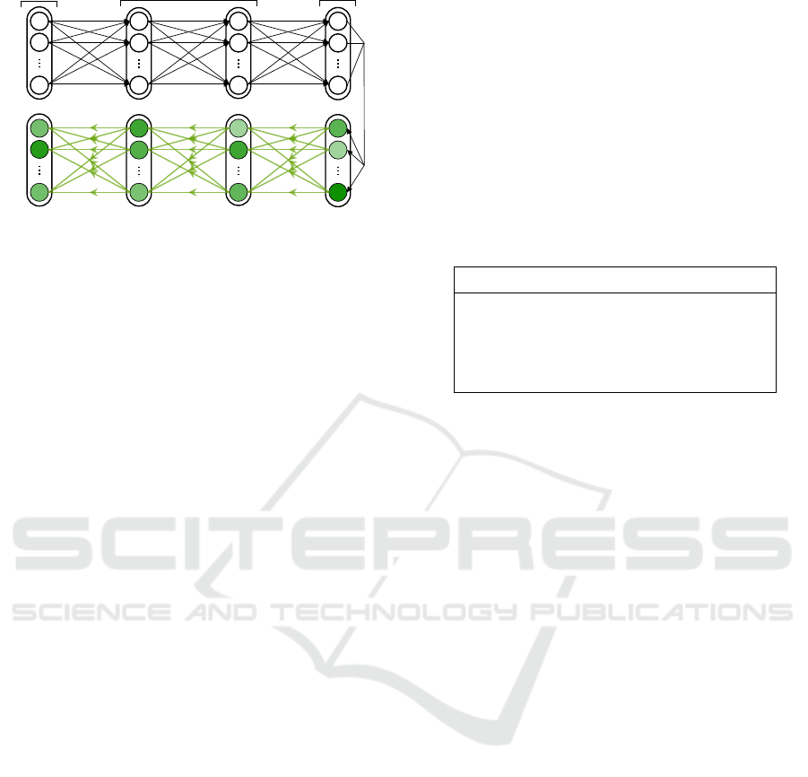
4.4 Generating SR Explanations
For each feature set, the respective trained model is
used to generate relevance charts. Figure 2 shows the
redistribution procedure for a model with two hidden
layers. Here, an input is first fed into the neural network
and propagated forward, storing the activations at each
stage. Once all layer activations are obtained, relevance is
redistributed according to one of the
LRP
rules described
in Table 2. The choice of rule depends on the input
domain. Here, we use four rule sets:
LRP
-
ε
(with
ε
set to 1e-7),
LRP
-
α
1
β
0
,
LRP
-
α
2
β
1
and deep Taylor
decompositions utilizing the
z
+
-rule for hidden layer
(ReLU) activations and the w
2
-rule for the input layer.
Charts are generated both globally (over all labels) as
well as on a per-label basis to explore the different decom-
positions and the quality of the explanations. Instance
decompositions are aggregated to produce a single more
generalized explanation (discussed further in Section 4.5).
4.5 Practical Considerations
Since each instance would be decomposed into a seperate
set of relevance measures, a method for systematically
aggregating relevance measures across instances was
required. For multi-label problems, each model output
is independent of the other outputs. Since we are using
sigmoid activations at the output layer, we know that
each output should be in the range
(0,1)
, with higher
values denoting a higher probability of the label being
present. By filtering relevance for a single label (i.e.
decomposing a single output by treating all other outputs
Explaining Spatial Relation Detection using Layerwise Relevance Propagation
381
24
20
17
31
input
explanation
output
scores
R
(2)
24
R
(3)
20
R
(3)
1
R
(3)
2
R
(2)
1
R
(2)
2
output layer
input layer
hidden layers
a
(2)
24
a
(2)
2
a
(2)
1
Figure 2: The redistribution process for a sample network.
Given a neural network and an input, the input is first
propagated forward through the network, storing the activations
at each layer for use in the next step. The last layer activations
(the output scores), are set as the relevance scores for the last
layer, and used as the base for relevance redistribution. Using
the redistribution rules, relevance is redistributed back along the
network, layer by layer, until the input layer relevance scores
are obtained. This is treated as our explanation.
as zeros), we can obtain the label relevance for that
instance. Due to relevance conservation, we know that
the sum of the input relevances is equal to the output
value for that label. We also know that larger values at
the output indicate a higher chance of a good prediction
and should therefore bear more weight compared to
smaller outputs. So, knowing that each instance’s input
relevance measures are implicitly weighted by the model
output, summing these up should present a weighted total
relevance measure for a given label. Normalizing this
weighted total relevance such that each class explanation
sums to one gives us a quantitative way to directly
compare relevance measures between classes.
This technique for aggregating relevance across
instances was used to generate relevance charts represen-
tative of all (true) positive predictions for a given label.
It was noted that the relevance charts for different labels
were still quite similar for certain classes. When pooling
language feature relevance measures, the large number
of features being pooled ends up saturating the relevance
such that most of the relevance is allocated to the pooled
feature. Hence, a weighted normalized mean explanation
common to all classes was created by summing up all the
relevance redistributions of all classes and instances (i.e.
before normalization) and then normalizing the sums. By
centering each label’s weighted total relevance according
to the weighted normalized mean relevance, we get more
informative explanations which take into account the
pooling bias. This technique was tested on a synthetic
dataset with a one-to-one correspondence between each
feature and each output class in order to verify that
explanations produced would be of a better quality.
5 RESULTS
5.1 Model Metrics
Table 3 shows the model metric scores for the best models
obtained by the
HPO
procedure, when evaluated over the
unseen test set. There are many possible justifications
as to why model accuracy did not exceed 0.6 for any of
our models. It could be that the architecture used here
Table 3: Model metric scores for the test set (per-instance accu-
racy and micro-averaged F
1
, precision and recall - higher is bet-
ter), for each feature set combination (G denotes geometric fea-
tures, D denotes depth features and L denotes language features).
Features Acc. F
1
Prec. Rec.
G 0.457 0.595 0.651 0.549
G+D 0.540 0.660 0.694 0.630
G+L 0.525 0.640 0.684 0.601
G+L+D 0.554 0.673 0.728 0.626
is not complex enough to represent the required function.
It could also be the imbalance in the dataset or that the
dataset is not large enough for the models to learn and
generalize.
The addition of depth features to the model had the
largest relative increase in accuracy. The inclusion of geo-
metric, language and depth features together did not have
a very significant increase in accuracy over the geometric
and depth features model performance. This may be
indicative of the fact that language and depth features may
provide redundant information for certain labels (individ-
ually, both are useful when added to the base geometric
features but, when combined together, the improvement
over the individual scenarios is less prominent). The gen-
eral trend with regards to precision and recall is that about
70% of the models’ positive predictions are correct and
the models manage to recall about 60% of positive labels.
5.2 Explaining Model Decisions
Despite the low accuracy scores, we can still generate
explanations by selecting only inputs from the test set
which produced true positive predictions for a given
label. Furthermore, by filtering relevance to only allow
relevance from that label to flow through, we get less
noisier (more consistent) explanations. Since the model
incorporating geometric, language and depth features has
the best performance, as well as a larger array of features
which may be useful for differentiating between
SR
s, the
main results shown here will be for this model.
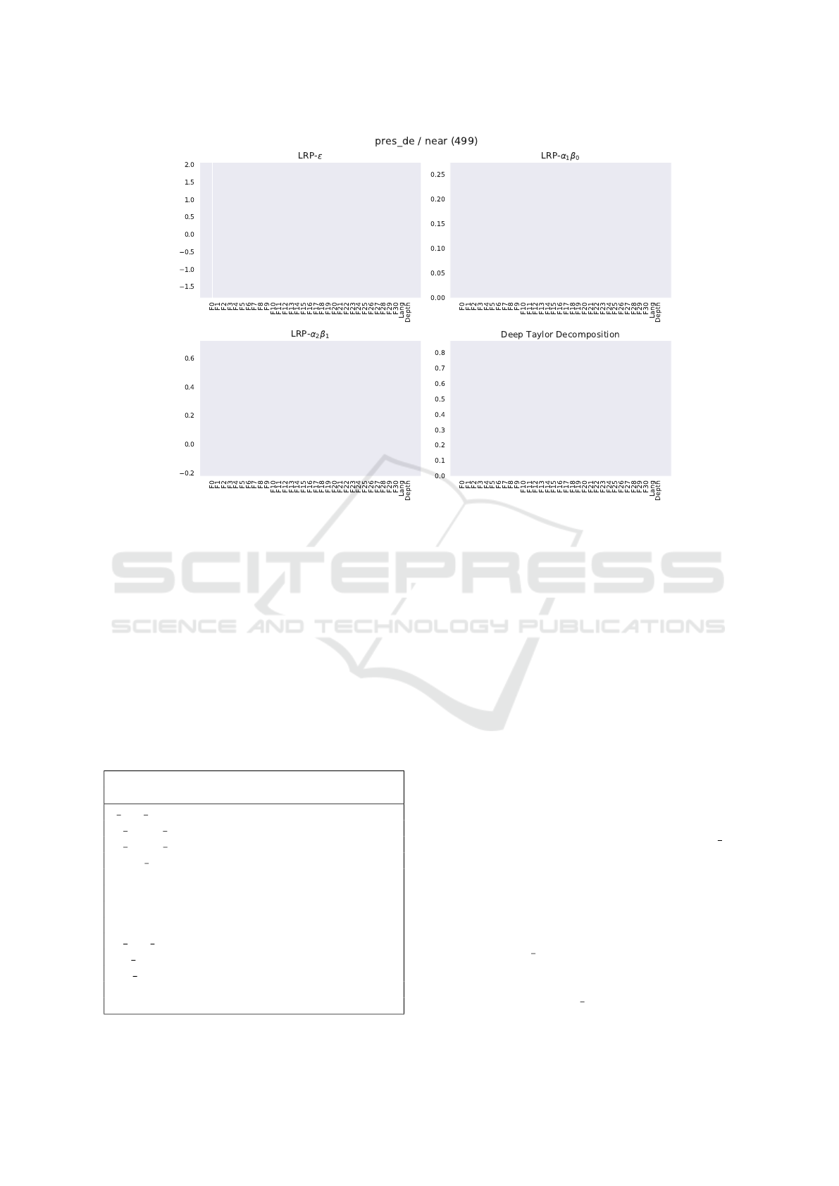
To illustrate the differences between the four
decomposition techniques, a single
SR
was decomposed
using each of them. Figure 3 shows these decompositions
side by side for comparison. It is immediately visible
VISAPP 2020 - 15th International Conference on Computer Vision Theory and Applications
382
Features Features
Relevance Relevance
Figure 3: Different explanations for the same preposition (near) using the geometric, language and depth features model, aggregated
over all positive instances. Comparing the outputs we see that the language features are chosen as highly relevant by all redistribution
techniques. However, the explanation produced by LRP-ε differs from the other explanations.
that the language features (which have been pooled into a
single measure) are usually dominant over other features.
This is the case for most labels as the pooling effect ends
up gathering a large portion of the relevance scores into
Table 4: Most relevant features when
LRP
-
α
1
β
0
is used for
decompositions, for each Spatial Relation, ranked by relevance
(top 3 shown). # refers to the number of classified instances
for that Spatial Relation. L denotes language features, D
denotes depth features and F0-F30 denote geometric features.
The results for derriere (behind) and devant (in front), which
both involve depth, show that
LRP
produces some promising
explanations.
Rank
Spatial Relation # 1 2 3
a cote de (beside) 242 F3
F15 F27
au dessus de (above) 2
F19 F12 F18
au niveau de (at the level of) 146 F5
F20 F15
autour de (around) 2 F1 F0 L
contre (against) 26 F5
F11 F12
dans (in) 5
F19
F5
F30
derriere (behind) 159 D
F18 F28
devant (in front) 150 D
F30 F28
en face de (opposite) 2 D
F12 F10
loin de (far from) 52 D
F18 F13
pres de (near) 499 L
F23 F22
sous (under) 69 L F1
F11
sur (on) 68
F11 F30
L
one feature. To mitigate this, the centered weighted total
relevance (centered by the weighted normalized mean
relevance) will be used.
Preliminary results show that
LRP
-
ε
is littered with
negative relevance.
LRP
-
α
2
β
1
also contains some
negative relevance, but only to a point where it does not
outweigh the positive elements in the explanation. As
expected,
LRP
-
α
1
β
0
and deep Taylor decompositions
contain only positive relevance measures. When center-
ing the weighted normalized mean explanation, a more
specific description of each class is obtained. As can be
seen in Figure 4, language and depth features are now less
prominent (since we’re taking into account the pooling
bias introduced in their favor). Table 4 summarizes the
results shown in Figure 4 by displaying the top three
relevant features for each class (after centering).
Looking at the most relevant features for pres de
(near), we see that the language features are ranked first.
Since the dataset contains a number of images of people
and in most images people are photographed with other
people (21.9% of the dataset contains persons as both
the trajector and landmark), a bias is present toward
that combination when at least one person is present.
Furthermore, pres de is marked as a true label for 66.4%
of the instances where two persons are present. This
means that the language features are probably being
marked as relevant for pres de due to this pattern.
Explaining Spatial Relation Detection using Layerwise Relevance Propagation
383

Features
Features
Relevance
Relevance
Relevance
Figure 4: Difference of
LRP
-
α
1
β
0
explanations from the weighted normalized mean explanation, for the most frequently predicted
prepositions. Note the relevance attributed to depth for derriere and devant, as well as the importance of language in predicting pres de.
Similarly, for sous (under), 71.5% of landmarks are
people and for sur (on), 79.4% of trajectors are peo-
ple. Compared with spatials such as derriere, devant
and loin de where the proportions of trajectors and land-
marks which are people are significantly smaller (37.7%
and 36.5%, respectively, at most), we can see that the
language features are only relevant for relations which
involve an exploitable pattern influenced by the nature of
the objects themselves.
Looking at the most relevant features as chosen by
deep Taylor decomposition (Table 5), we now see that
language features, depth features or both are chosen as
relevant in all but three cases. For a cote de (beside) and
au niveau de (at the level of), F18 (an indicator of dif-
ference in upper edge height between the two objects) is
chosen as the most relevant feature. This could be viewed
as a requirement for the two objects to have an aligned up-
per edge. F3 and F20 are also common among a cote de
and au niveau de but are harder to make sense of as they
all describe areas of some form. It is clear that intuitive
explanations can be extracted for some features but other
features appear to be less directly related with the concepts
for which they are relevant. With that being said, for the
purposes of extracting even more intuitive explanations
it might be a good idea to restrict the set of geometric fea-
tures to more basic features, primitives, which can be im-
mediately made sense of. Having knowledge of which fea-
tures the neural network is paying attention to in the pre-
diction of
SR
s facilitates the process of comparing human
decisions with those of machine learnt models, thus ad-
vancing both automation as well as artificial intelligence.
VISAPP 2020 - 15th International Conference on Computer Vision Theory and Applications
384

Table 5: Most relevant features using deep Taylor decompo-
sition, for each Spatial Relation, ranked by relevance (top 3
shown). # refers to the number of classified instances for that
Spatial Relation. L denotes language features, D denotes depth
features and F0-F30 denote geometric features.
Rank
Spatial Relation # 1 2 3
a cote de (beside) 242
F18
F3
F20
au dessus de (above) 2
F12
L F1
au niveau de (at the level of) 146
F18
F3
F20
autour de (around) 2 L F0
F23
contre (against) 26 F5
F23 F14
dans (in) 5 L
F30 F23
derriere (behind) 159 D L
F21
devant (in front) 150 D
F30
F5
en face de (opposite) 2 D L
F30
loin de (far from) 52 D
F30 F28
pres de (near) 499 L
F13 F12
sous (under) 69 L D
F24
sur (on) 68 L D
F30
6 CONCLUSIONS
We can conclude that
LRP
is useful for generating human-
interpretable explanations. This is partly due to the fact
that some of the geometric features lend themselves
to human-understandable terms, for example distance
between objects, whereas others, although they are not
terms used by human beings, are one step away from be-
ing so. For example, area overlap of bounding boxes can
act as a proxy to occlusion and to a lesser extent to depth.
The results show that language is important for
some prepositions but not for others, which concur with
observations from the cognitive linguistics literature
(Dobnik et al., 2018). On the other hand, it’s hard to
isolate a single feature as the most relevant, since feature
relevance was seen to be class-dependent. By employing
the centering approach a feature ordering in terms of
relevance was defined for each class. Applying the
relevance redistribution techniques described here to a
SRD
problem is a process which has not been carried out
before and allowed us to study the importance of features
per-class rather than globally. Additionally, we confirm
that depth features are important for some
SR
s and it
is therefore useful to have access to depth features in
addition to bounding boxes. In the future we plan to ex-
tend this study to more varied datasets and to analyze the
quality of explanations quantitatively, for example using
feature removal or inversion as in (Bach et al., 2015).
REFERENCES
Bach, S., Binder, A., Montavon, G., Klauschen, F., M
¨
uller,
K.-R., and Samek, W. (2015). On pixel-wise explanations
for non-linear classifier decisions by layer-wise relevance
propagation. PLoS One.
Belz, A., Muscat, A., Aberton, M., and Benjelloun, S. (2015).
Describing Spatial Relationships between Objects
in Images in English and French. pages 104–113.
Association for Computational Linguistics.
Belz, A., Muscat, A., Anguill, P., Sow, M., Vincent, G., and
Zinessabah, Y. (2018). SpatialVOC2K: A Multilingual
Dataset of Images with Annotations and Features for
Spatial Relations between Objects. Technical report.
Coventry, K. R., Prat-Sala, M., and Richards, L. (2001).
The Interplay between Geometry and Function in the
Comprehension of Over, Under, Above, and Below. J.
Mem. Lang.
Dai, B., Zhang, Y., and Lin, D. (2017). Detecting visual
relationships with deep relational networks. In Proc. -
30th IEEE Conf. Comput. Vis. Pattern Recognition, CVPR
2017, volume 2017-Janua, pages 3298–3308.
Dobnik, S., Ghanimifard, M., and Kelleher, J. (2018). Exploring
the Functional and Geometric Bias of Spatial Relations
Using Neural Language Models.
Dobnik, S. and Kelleher, J. (2015). Exploration of functional
semantics of prepositions from corpora of descriptions
of visual scenes.
Elliott, D. and Keller, F. (2013). Image Description using Visual
Dependency Representations. Technical report.
Gevrey, M., Dimopoulos, I., and Lek, S. (2003). Review and
comparison of methods to study the contribution of vari-
ables in artificial neural network models. In Ecol. Modell.
Hashem, S. (1992). Sensitivity analysis for feedforward
artificial neural networks with differentiable activation
functions. In Proc. 1992 Int. Jt. Conf. Neural Networks.
Lu, C., Krishna, R., Bernstein, M., and Fei-Fei, L. (2016).
Visual relationship detection with language priors. In
Lect. Notes Comput. Sci. (including Subser. Lect. Notes
Artif. Intell. Lect. Notes Bioinformatics), volume 9905
LNCS, pages 852–869.
Montavon, G., Lapuschkin, S., Binder, A., Samek, W., and
M
¨
uller, K.-R. (2017). Explaining nonlinear classification
decisions with deep Taylor decomposition. Pattern
Recognit.
Muscat, A. and Belz, A. (2017). Learning to Generate Descrip-
tions of Visual Data Anchored in Spatial Relations. IEEE
Comput. Intell. Mag., 12(3).
Ramisa, A., Wang, J., Lu, Y., Dellandrea, E., Moreno-Noguer,
F., and Gaizauskas, R. (2015). Combining geometric,
textual and visual features for predicting prepositions in
image descriptions. In Conf. Proc. - EMNLP 2015 Conf.
Empir. Methods Nat. Lang. Process., pages 214–220.
Association for Computational Linguistics.
Ribeiro, M. T., Singh, S., and Guestrin, C. (2016). Model-
Agnostic Interpretability of Machine Learning.
Zhu, Y. and Jiang, S. (2018). Deep structured learning for
visual relationship detection. In 32nd AAAI Conf. Artif.
Intell. AAAI 2018, pages 7623–7630.
Explaining Spatial Relation Detection using Layerwise Relevance Propagation
385
