Comparison of Continuous and Discontinuous Charging Models for the

Electric Bus Scheduling Problem

Maros Janovec

and Michal Kohani

Faculty of Management Science and Informatics, University of

Zilina, Univerzitn

a 8215/1, 010 26

Zilina, Slovakia

Keywords:

Electric Buses, Scheduling Problem, Exact Approach, Discontinuous Charging.

Abstract:

Electric buses offer an alternative to conventional vehicles in the public transport system due to their low

operational costs and low emissions. Therefore, the standard problems must be resolved with respect to the

nature of the electric buses, which is mainly the reduced driving range and charging time. In this paper, we

deal with the electric bus scheduling problem. We propose changes to the previously presented model, which

allowed only the continuous charging. These changes will allow the model to describe also discontinuous

charging when the electric bus can be unplugged during the charging, then let another electric bus to charge

and after that plug-in to charger again. These two formulations are tested by IP solver and the solutions

and performance of both discontinuous charging and continuous charging formulations are compared on the

datasets generated from the data provided by public transport system provider DPM

Z in the city of

Zilina.

1 INTRODUCTION

In recent years the importance of electric vehicles is

increasing. The countries are trying to improve the

ecology and therefore reduce the emissions. The elec-

tric vehicles are a way that can reduce CO

emissions.

From the point of public transport system providers,

the use of electric vehicles can reduce operational

costs.

With the application of the electric vehicles in the

public transport system, different problems must be

addressed. These problems are for example line plan-

ning, vehicle, and crew scheduling. The electric vehi-

cles have reduced driving range, based on the capac-

ity of the battery and also the charging time must be

considered, because it is much longer than the time

needed to refuel a conventional vehicle. Due to these

facts, the problems must be remodeled and new meth-

ods to solve these problems need to be proposed.

In our paper, we address the electric bus schedul-

ing problem (EBSP) which is a special case of vehi-

cle scheduling problem with the constraints of energy

and driving range. In this problem, we are assigning

electric buses to service trips, that need to be served.

In this paper, we are proposing changes to our pre-

viously presented mathematical model (Janovec and

https://orcid.org/0000-0002-0370-8560

https://orcid.org/0000-0002-9421-4899

Koh

ani, 2019b; Janovec and Koh

ani, 2019a) which

allowed only continuous charging, that would enable

discontinuous charging. That means during the charg-

ing the unplugging is possible and then after an inter-

val of waiting the bus can be plugged in again and

continue charging. The discontinuous charging has

the potential to improve some types of objectives like

minimizing the charged energy but can worsen solu-

tions of different objectives like time spent waiting.

In this paper, we are researching the objective of min-

imizing the number of used electric buses. Due to

the complexity of the EBSP, we do not consider the

schedule of the drivers, therefore we assume that the

bus can be driven by different drivers and it is possible

to change drivers during the duty of the electric bus.

The proposed model is tested with an IP solver

on several datasets to ﬁnd if discontinuous charging

changes the results obtained by the continuous charg-

ing model and the changes in the computational time.

In section 2 the state-of-the-art in the ﬁeld is men-

tioned. Then in section 3 the problem of scheduling

electric buses is described and a linear mathematical

model for continuous charging is mentioned. Also,

the changes to the model that would enable discontin-

uous charging are proposed in this section. In section

4 the numerical experiments are described and the re-

sults we obtained are discussed. The last section con-

cludes the research and suggests possible future pos-

sibilities.

Janovec, M. and Kohani, M.

Comparison of Continuous and Discontinuous Charging Models for the Electr ic Bus Scheduling Problem.

DOI: 10.5220/0008962901790186

In Proceedings of the 9th International Conference on Operations Research and Enterprise Systems (ICORES 2020), pages 179-186

ISBN: 978-989-758-396-4; ISSN: 2184-4372

179

2 RELATED WORK

The vehicle scheduling problem is a well-researched

problem and a lot of variants are known. Some

basic ideas on how the vehicle scheduling problem

is modeled and solved were mentioned in (Bunte

and Kliewer, 2009). There the authors present an

overview of the models for a single depot vehicle

scheduling problem as well as models for a multi-

ple depot scheduling problem. The basic ideas, how

the problem is solved, are mentioned for each model.

The authors also present different extensions of the

vehicle scheduling problem, like heterogeneous ﬂeet,

time windows and route constraints. All these exten-

sions make the scheduling an NP-hard problem, but

for some speciﬁc cases, polynomial algorithms exist.

One example is a two depot vehicle scheduling prob-

lem, for which a speciﬁc solution method based on the

graph theory was proposed in (Czimmermann, 2006).

The scheduling of electric vehicles has two direc-

tions based on the used technology, speciﬁcally the

battery exchange system and the electric bus charg-

ing system. The scheduling with the battery exchange

system was addressed in (Kim et al., 2015) where the

authors proved the usability of the system by simula-

tion from the data gathered during an experimental

application of the electric buses in Soul. Schedul-

ing of electric buses with the battery exchange sys-

tem was researched by (Chao and Xiaohong, 2013),

where the authors present a mathematical model for

the single depot vehicle scheduling problem with two

objective functions. This problem was solved by the

Non-Dominated Sorting Genetic Algorithm.

The bus charging system is speciﬁc by charging

the buses during their operation or during the night

in the depot. The scheduling problem for this tech-

nology was addressed in (Sassi and Oulamara, 2017),

where a linear mathematical model for the schedul-

ing problem was presented. Besides the standard con-

straints of the battery, the model includes constraints

of maximal charging power that can be obtained from

the power grid. The authors also proposed two heuris-

tic algorithms to solve the problem and proved the

NP-hardness of the electric bus scheduling problem.

Next, two mathematical models were proposed by

(van Kooten Niekerk et al., 2017). The ﬁrst model as-

sumed that charging is a linear process and the second

model was able to describe also a non-linear charging

process by discretization of the battery energy state.

The proposed models were solved by exact methods

and by the column generation method.

Non-linear model for the electric bus schedul-

ing problem was presented by (Rogge et al., 2018)

and was solved by grouping genetic algorithm. This

model considered only charging at one location,

speciﬁcally the depot. Also, the electric bus always

charges to the maximum capacity.

All of the above-mentioned authors who re-

searched the electric bus scheduling problem with bus

charging technology assumed the bus is charging con-

tinuously. Therefore, we focus on the discontinuous

charging, where the bus can be unplugged during the

charging and then again plugged-in after some time

of not charging. The possible advantages of this ap-

proach to charging electric vehicles were mentioned

in (Yanjin et al., 2016).

3 PROBLEM DESCRIPTION

In the problem of the electric bus scheduling prob-

lem (EBSP) we assign available electric buses to the

tasks that need to be served, which create a schedule

for each electric bus. The schedule is composed of

two different tasks (Fig. 1). The ﬁrst type of task is

serving a service trip, which is a required type of task.

The second type of task is charging, when the electric

bus is plugged into a charger and it charges the bat-

tery. This type of task is voluntary and is performed

only when needed.

Figure 1: Illustration of electric bus schedules with arcs

connecting tasks of one electric bus schedule and arcs con-

necting charging events on one charger.

Each schedule of electric buses must met certain

conditions to be called feasible. The most important

condition is that each service trip is assigned to one

electric bus. Also, the electric bus can not be assigned

to more trips simultaneously. Furthermore, due to the

nature of electric buses, we add conditions that the bus

must have enough energy during the whole schedule

and that the battery capacity can not be exceeded dur-

ing the charging.

ICORES 2020 - 9th International Conference on Operations Research and Enterprise Systems

180

3.1 Formal Formulation of the Problem

In the models, we use the set N of all the service trips.

Next, we add the depot, where the morning depot is

represented by the node D

and the evening depot is

represented by the nodes D

, where we add one pos-

sible depot node for each service trip. The set R is a

set of all chargers. At each charger r ∈ R we have T

charging events, which are time intervals. Lastly, the

set of all electric bus types is denoted as K.

Each service trip i ∈ N is deﬁned by the start time

and its duration t

. The energy consumption during

the trip is denoted as constant c

. Next, the constant t

i j

represents the time of transfer between the end termi-

nal of trip i and the start terminal of the trip j. The en-

ergy consumed during this transfer trip is represented

by constant c

i j

A charger r ∈ R has its charging speed q

deﬁning

how much energy is charged during one unit of time.

The next needed information about the charger is its

location. This is represented by the travel time be-

tween the end terminal of service trip i and the charger

r denoted as t

with the energy consumption of c

Location is also deﬁned by the travel time t

r j

between

the charger r and the starting terminal of service trip

j with the energy consumption of c

r j

At each charger r we deﬁned a set of charging

events T

. Each charging event is derived from the

service trip. In other words, we create a charging

event on each charger for every service trip. The

charging event t at charger r is characterized by its

starting time s

, which is connected to the corre-

sponding service trip and is deﬁned as s

= s

where s

is starting time of corresponding service trip,

is its duration and t

is the transfer time between the

trip and the charger. Also, the charging events in the

set T

at charger r ∈ R are ordered by ascending start-

ing time, which divides the whole available charging

time into intervals with different length

An available electric bus type k ∈ K is character-

ized by its battery. The battery has maximal capacity

represented by constant SoC

max

for each bus type k.

We also deﬁne a minimal battery capacitySoC

min

for

each bus type k, which can be used as the minimum

reserve of energy.

3.2 Mathematical Models

In this section, we list both of the linear mathemat-

ical models for the problem of scheduling of electric

buses. The ﬁrst model is speciﬁc by continuous charg-

ing and the second represents also the alternative of

the discontinuous charging.

3.2.1 Continuous Charging Model

This model was presented in our previous work

(Janovec and Koh

ani, 2019a; Janovec and Koh

ani,

2019b), and there only continuous charging is en-

abled. That means the electric bus after plugging-in

to charger can start charging, but after unplugging, the

bus must continue to serve a service trip.

In this model we use sets F

, B

, Fc

, Bc

for each

charger i ∈ N, which are used to reduce the number

of the decision variables. Set F

represent all possi-

ble following service trips, to which the electric bus

can transfer after the end of the service trip i. In other

words for trip j to be in set F

of trip i the condition

≥ s

must hold, where s

is starting time of ser-

vice trip j, s

is starting time of trip i and t

is duration

of service trip i. Similarly the set B

is a set of all

possible previous service trips to trip i.

The set Fc

is connected to charging events and

it contains the charging events at charger r which can

be visited after ﬁnishing the service trip i. For each

charging event t ∈ T

at charger r ∈ R in the set Fc

the condition s

≥ s

+ t

must hold, where s

is starting time of charging event t at charger r, s

is starting time of trip i, t

is duration of trip i and

is transfer time between ending point of trip i and

charger r. Similarly the set Bc

is a set of all possible

previous charging events at charger r of service trip i,

for which the condition s

≤ s

is true, where t

is transfer time from the charger r to the starting point

of trip i.

For each charging event t at charger r the set

Fi(r, t) deﬁne the following service trips and set

Bi(r,t) deﬁne previous charging events. For trip i to

become a part of set Fi(r, t) the condition s

≤ s

must be satisﬁed. Similarly the condition s

≥ s

must hold for trip i to be in set Bi(r, t) of charg-

ing event t at charger r.

Next, we deﬁne the decision variable x

i j

which de-

scribes the decision to serve the service trip j just af-

ter serving service trip i with the vehicle k. The next

variables y

irt

and z

rt j

are connected to the transfer to

and from charger. Variable y

irt

represents the transfer

from the end terminal of service trip i to the charger

r to charge during the charging event t with the vehi-

cle k. The transfer from the charger r after charging

during charging event t to the starting terminal of ser-

vice trip j by the vehicle k is represented by decision

variable z

rt j

The variable w

represents the principle of contin-

uous charging. The variable represents the decision

to continue charging during the following charging

event t + 1 which begins just after the end of charg-

ing event t at charger r with the vehicle k.

Comparison of Continuous and Discontinuous Charging Models for the Electric Bus Scheduling Problem

181

To keep track of the energy state of the battery in

each used electric bus the last two variables e

and

are introduced. The variable e

is energy state of

bus k just before the service trip i. The variable ε

similar, but it represent the energy state of bus k just

before the start of charging event t at charger r.

Objective

minimize

∑

k∈K

∑

j∈F

∑

k∈K

∑

r∈R

∑

t∈Fc

(1)

The objective function (1) minimizes the number

of used electric buses, where the ﬁrst sum is the num-

ber of electric buses that depart from depot to the ser-

vice trip and the second sum is the number of electric

buses that depart from depot to the charger.

Vehicle Scheduling Constraints

∑

k∈K

∑

i∈B

i j

∑

k∈K

∑

r∈R

∑

t∈Bc

r j

rt j

= 1 ∀ j ∈ N (2)

∑

k∈K

∑

j∈Bi

jrt

∑

k∈K

rt−1

≤ 1 ∀ r ∈ R, t ∈ T

(3)

∑

i∈B

i j

∑

r∈R

∑

t∈Bc

r j

rt j

∑

l∈F

∑

r∈R

∑

t∈Fc

r j

jrt

∀ j ∈ N, k ∈ K (4)

∑

i∈Bi

irt

+ w

rt−1

∑

j∈Fi

rt j

+ w

∀ r ∈ R, t ∈ T

, k ∈ K (5)

To ensure that each service trip is served the con-

ditions (2) are used. The constrains (3) are connected

with a condition that during one time interval only

one electric bus can be charged at the charger. The

constraints (4) are standard ﬂow constraints that en-

sure the same bus which was assigned to serve the

service trip would be assigned to serve the next task.

The constraints (5) are ﬂow constraints also, but they

are connected to the charging events. That means the

bus which arrived to charge during a charging event

also leaves to serve a service trip or continue to charge

during the next interval after the end of the charging

event.

Energy Consumption Constraints

= SoC

max

∀ k ∈ K (6)

≥ SoC

min

+ c

∑

j∈F

i j

∑

r∈R

∑

t∈Fc

irt

∀ i ∈ N, k ∈ K (7)

+ c

r j

+ Mq

(1 − z

rt j

) ≥ SoC

min

+ z

rt j

r j

∀ r ∈ R, t ∈ T

, k ∈ K, j ∈ Fi

(8)

≤ e

− x

i j

+ c

i j

) + SoC

max

(1 − x

i j

)

∀ j ∈ N, i ∈ B

, k ∈ K (9)

≥ e

− x

i j

+ c

i j

) − SoC

max

(1 − x

i j

)

∀ j ∈ N, i ∈ B

, k ∈ K (10)

≤ e

− y

irt

+ c

) + SoC

max

(1 − y

irt

)

∀ r ∈ R, t ∈ T

, k ∈ K, i ∈ Bi

(11)

≥ e

− y

irt

+ c

) − SoC

max

(1 − y

irt

)

∀ r ∈ R, t ∈ T

, k ∈ K, i ∈ Bi

(12)

The constraints (6) initialize the battery capacity

to the maximum before the start of the working day

for each electric bus. To ensure the bus has enough

energy to drive the service trip and the following

transfer the constraints (7) are used. In these con-

straints, the constant SoC

min

is used as a lower limit of

the battery energy state, which can be understood as

the energy reserve of the battery. A similar condition

is represented by the constraints (8), which ensures

the bus has enough energy to transfer to the following

service trip after the charging.

One of the conditions which must be satisﬁed is

the energy preservation. To ensure this condition the

constraints (9) - (12) are introduced. The preservation

of energy between two consecutive service trips is de-

ﬁned by a pair of constraints (9) and (10). The next

pair of constraints (11) and (12) preserve the energy

between the service trip and the following charging

event.

Charging Constraints

+ c

r j

− ε

+ SoC

max

(1 − z

rt j

) ≥ 0

∀ r ∈ R, t ∈ T

, k ∈ K, j ∈ Fi

(13)

rt+1

− ε

+ SoC

max

(1 − w

) ≥ 0

∀ r ∈ R, t ∈ T

, k ∈ K (14)

+ c

r j

− Mq

(1 − z

rt j

) ≤ SoC

max

∀ r ∈ R, t ∈ T

, k ∈ K, j ∈ Fi

(15)

rt+1

− Mq

(1 − w

) ≤ SoC

max

∀ r ∈ R, t ∈ T

, k ∈ K (16)

ICORES 2020 - 9th International Conference on Operations Research and Enterprise Systems

182

≤ ε

+ z

rt j

((s

−t

r j

− s

− c

r j

)

+ SoC

max

(1 − z

rt j

)

∀ j ∈ N, r ∈ R,t ∈ Bc

r j

, k ∈ K (17)

rt+1

≤ ε

+ w

rt+1

− s

+ SoC

max

(1 − w

)

∀ r ∈ R, t ∈ T

, k ∈ K (18)

+ c

r j

− ε

− SoC

max

(1 − z

rt j

) ≤ (s

rt+1

− s

∀r ∈ R, t ∈ T

, k ∈ K, j ∈ Fi

(19)

The constraints (13) and (14) serves as a limitation

that the charged energy must be non-negative. Simi-

larly, the constraints (15) and (16) deﬁne the upper

bound of the battery energy state, which means the

maximal capacity of the battery is not exceeded dur-

ing the charging. Speciﬁcally, constraints (13) and

(15) are connected to a charging event which is fol-

lowed by the service trip and the constraints (14) and

(16) are connected to charging event followed by the

next charging.

The next constraints (17), (18) and (19) limit the

available charging time based on the decisions. It is

deﬁned that the ending time of the charging event is

variable. But the time is limited by the start of the fol-

lowing service trip if the bus continues to the service

trip after charging, which is represented by the con-

straints (17). The charging time is also limited by the

start of the next charging event. This is represented by

the constraints (18) and (19). The constraints (18) are

applied when the charging event is followed by a next

charging event and constraints (19) are used when the

charging event is followed by a service trip.

Integrality and Non-negativity Constraints

i j

∈ {0, 1} ∀ k ∈ K, i ∈ N ∪ D

∪ D

, j ∈ F

(20)

irt

∈ {0, 1} ∀ k ∈ K, i ∈ N, r ∈ R, t ∈ Fc

(21)

rt j

∈ {0, 1} ∀ k ∈ K, r ∈ R, t ∈ T

, j ∈ Fi

(22)

∈ {0, 1} ∀ k ∈ K, r ∈ R, t ∈ T

(23)

≥ 0 ∀ k ∈ K, i ∈ N (24)

≥ 0 ∀ k ∈ K, r ∈ R, t ∈ T

(25)

The constraints (20), (21), (22) and (23) deﬁne the

decision variables x

i j

, y

irt

, z

rt j

and w

are binary. Fi-

nally, the non-negativity of the variables e

and ε

that keep track of the energy state, is deﬁned in the

constraints (24) and (25).

3.2.2 Discontinuous Charging Model

In this section, we propose changes to the model,

which would enable discontinuous charging. That

means the electric bus can be unplugged after charg-

ing during one time interval at charger, then wait

during the following time interval and at last can be

plugged again during the next time interval without

the need to continue by serving a service trip. The

change is shown in ﬁgure 2.

Figure 2: Difference between the continuous (a) and dis-

continuous (b) charging.

To deﬁne the connection between different charg-

ing events we introduce new decision variable u

rts

which represent decision that the electric bus k will

continue charging at charger r during the charging

event s after the charging during the charging event t.

To reduce the number of decision variables and also to

deﬁne only variables which are feasible from the time

point of view the set is introduced. The charging event

s to become a part of a set set C f

deﬁned for charger

r and charging event t the charging event is s must

be on the same charger as event t and the condition

<= s

must hold. In our case we have the charg-

ing events sorted by the starting time at each charger,

that means in the set C f

are all the events that follow

the charging event t, or we can write s ∈ t +1, ...|T

Similarly, the set of previous charging events Cb

deﬁned. It includes all the charging events that have

a start time before the start of the charging event t at

charger r.

With variable u

rts

we replace the variable w

from

the continuous model and also adjust some of the con-

straints of the continuous charge model to consider

not only the following, respectively previous charg-

ing event, but all the following, respectively previous

charging events. The adjustments are shown and de-

scribed below.

∑

k∈K

∑

j∈Bi

jrt

∑

k∈K

∑

s∈C f

rts

≤ 1 ∀ r ∈ R, t ∈ T

(26)

Comparison of Continuous and Discontinuous Charging Models for the Electric Bus Scheduling Problem

183

∑

i∈Bi

irt

∑

s∈Cb

rst

∑

j∈Fi

rt j

∑

p∈C f

rt p

∀ r ∈ R, t ∈ T

, k ∈ K (27)

The constraints (26) replace the constraints (3),

which ensures that during one time interval only one

electric bus can be charged. The adjustment lies in the

fact we need to consider not only the previous charg-

ing event but all of the previous charging events. With

this idea we adjusted also the ﬂow constraints (5) into

constraints (27), where we added into the constraints

all the connections between the current charging event

and previous, respectively following charging events.

We have not changed the energy consumption

constraints, because they do not depend on the con-

nections between the charging events.

− ε

+ SoC

max

(1 − u

rts

) ≥ 0

∀ r ∈ R, t ∈ T

, s ∈ C f

, k ∈ K (28)

− Mq

(1 − u

rts

) ≤ SoC

max

∀ r ∈ R, t ∈ T

, s ∈ C f

, k ∈ K (29)

≤ ε

+ u

rts

rt+1

− s

+ SoC

max

(1 − u

rts

)

∀ r ∈ R, t ∈ T

, s ∈ C f

, k ∈ K (30)

Constraints (14) were changed into constraints

(28), where we need to consider all combinations of

following charging events to set the charged energy

is non-negative. Similarly, the constraints (16) were

changed into constraints (29) and deﬁne the battery

does not exceed its maximal capacity during charg-

ing. The constraints (16) are added for each possi-

ble combination of charging events. Lastly the con-

straints (18) is changed into constraints (30) for each

possible combination of charging events. These con-

straints limit the charging time by the start of the im-

mediately following charging event. In this case, the

way we count the charged energy is changed.

rts

∈ {0, 1} ∀ k ∈ K, r ∈ R, t ∈ T

, s ∈ C f

(31)

The integrality constraints (31) deﬁne that the de-

cision variable u

rts

is binary and also replace the

obligatory constraints (23) of variable w

4 NUMERICAL EXPERIMENTS

To test the adjustments of the model we performed a

number of experiments. Also to compare the perfor-

mance of both models we compared the computation

time of the exact solution made by the standard IP

solver Xpress IVE. The experiments were performed

on the machine with Intel Core i5-7200U 2,5Ghz,

16GB of RAM.

4.1 Data Description

For the experiments, we used data provided by the

public transport system provider DPM

Z in the city of

Zilina. This data contains information about the ser-

vice trips of diesel buses performed during one day

of operation. To test the models we generated six

datasets that cover different bus lines and contain a

different number of service trips.

The ﬁrst dataset, denoted as DS1, contains 49 ser-

vice trips performed on line 26. The second dataset

(DS2) contains 77 trips served on line 27. The third

dataset (DS3) is a union of trips served on lines 26

and 29 and contains 83 trips. The fourth dataset (DS4)

covers lines 20, 29, 30 and 31 with 105 trips. The ﬁfth

dataset (DS5) covers lines 20, 26, 29 and 30 with 133

trips and the last dataset (DS6) is a union of 160 trips

served at lines 26, 27 and 29.

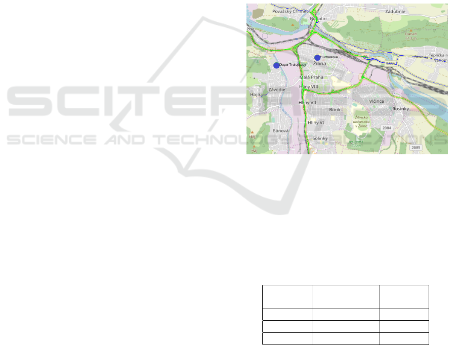
Figure 3: Locations of charger in the city of

Zilina.

The second needed part of the experiments is the

location of the chargers. In our experiments, we use

the current locations of chargers. There are two charg-

ers at the trolleybus depot and one charger at the cen-

ter of the city. These locations can be seen in ﬁgure 3

as blue dots.

Table 1: Energy consumption and battery capacity scenar-

ios.

Scenario

Energy

consumption

Battery

capacity

Spring 0,8 kWh/km 140 kWh

Summer 1,08 kWh/km 140 kWh

Winter 1,08 kWh/km 105 kWh

The last part of the experiments were different sce-

narios based on the time of the year, which represent

different maximal energy states and different energy

consumption. The scenarios are summed up in the ta-

ble 1. The ﬁrst scenario represents the basic setup. It

is connected to the spring and autumn season. The

ICORES 2020 - 9th International Conference on Operations Research and Enterprise Systems

184

battery capacity was set to 140kWh based on the lit-

erature (ZeEUS project, 2016). The second scenario

is a summer scenario with increased energy consump-

tion per km by 35%, which is caused by the running

of air condition. In the last scenario, the energy con-

sumption is increased by 35% and the capacity is de-

creased by 25%. This scenario represents the win-

ter season, where the energy is also consumed on the

heating and the battery has lower capacity due to the

low temperature (Wood et al., 2012; Millner, 2010).

4.2 Results

In the tables 2, 3 and 4 we can see results of the ex-

periments performed on all the datasets with each sce-

nario. In each table, we have two columns - Continu-

ous and Discontinuous. The column Continuous rep-

resents the results of continuous charging model and

column Discontinuous shows the results of the dis-

continuous charging model. For each model we have

the solution (Sol) obtained by the IP solver, then col-

umn BB represents best bound of the solution and col-

umn Time is the computational time in seconds. Also,

the results obtained by the continuous model were the

same as the solution of the classic VSP problem.

Table 2: Results of experiments with spring scenario.

Data-

set

Continuous Discontinuous

Sol BB Time Sol BB Time

DS1 4 4 3 4 4 4,4

DS2 4 4 12,2 4 4 36,6

DS3 5 5 35,6 5 5 49,9

DS4 6 6 29,7 6 6 64,3

DS5 8 8 169,2 8 8 222,6

DS6 9 9 281,6 9 9 507,7

Table 3: Results of experiments with summer scenario.

Data-

set

Continuous Discontinuous

Sol BB Time Sol BB Time

DS1 4 4 2,9 4 4 5,4

DS2 4 4 12 4 4 36

DS3 5 5 36,5 5 5 50,2

DS4 6 6 31,3 6 6 65,1

DS5 8 8 170,7 8 8 211,8

DS6 9 9 282,8 9 9 544,9

The table 2 represent the results of the spring sce-

nario. We can see that the results obtained by both

models are the same. However, the solution time is

different. The computational time needed for the dis-

continuous charging model is always higher than for

the continuous charging model. This is caused by the

fact, that the discontinuous charging model is more

Table 4: Results of experiments with winter scenario.

Data-

set

Continuous Discontinuous

Sol BB Time Sol BB Time

DS1 4 4 3,3 4 4 10,6

DS2 4 4 33,8 4 4 131,8

DS3 5 5 42,9 5 5 286,8

DS4 6 6 773,5 6 6 920

DS5 10 8 57600 11 8 57600

DS6 11 9 57600 13 9 57600

complex, therefore more time is needed to solve this

model.

The results of the summer scenario are listed in

table 3. Similar to spring scenario the results of both

models are the same and the computational time is

also higher for discontinuous charging model. If we

compare the computation time between the spring and

summer scenario, the times are not much different.

Therefore we can conclude that the energy consump-

tion does not have a high impact on the computation

time.

The last scenario is the winter scenario, which

results are listed in table 4. There, for the smaller

datasets, the optimal solutions were obtained for both

models. In the case of datasets DS5 and DS6, the op-

timal solution was not found in the time limit, which

was set to 16 hours. There we can see that the so-

lution obtained by the continuous charging model is

Table 5: Number of used charging intervals (UCI), multi-

ple interval charging events (MIC) and interrupted charging

events (IC) for continuous and discontinuous charging in

spring (Sp), summer (Su) and winter(Wi) scenario (SC).

Data-

set

Continuous Discontinuous

UCI MIC UCI MIC IC

DS1

Sp 3 0 6 1 0

Su 3 0 6 1 0

Wi 9 0 13 0 0

DS2

Sp 22 1 31 0 0

Su 22 1 31 1 0

Wi 36 4 51 13 0

DS3

Sp 42 3 32 1 0

Su 42 3 32 1 0

Wi 41 5 60 13 1

DS4

Sp 43 5 59 9 4

Su 43 5 59 9 4

Wi 84 17 70 14 0

DS5

Sp 62 4 65 10 2

Su 62 4 66 14 2

Wi 113 23 122 32 9

DS6

Sp 77 5 88 15 7

Su 77 5 88 15 7

Wi 157 36 146 35 16

Comparison of Continuous and Discontinuous Charging Models for the Electric Bus Scheduling Problem

185

better. As we mentioned before this is caused by the

increased complexity of the discontinuous charging

model. From the point of comparison of the solution

time between different scenarios, the winter scenario

has increased computation time for both models. This

is caused by the decreased capacity of the battery.

In the table 5, there is a comparison of the count

of the charging intervals that were used for charg-

ing (UCI) during a speciﬁc scenario for each dataset.

From the results, we cannot say which type of charg-

ing uses less charging intervals. However, a change

can be seen in the number of charging events that

took multiple intervals (MIC). There the continuous

charging uses usually less number of multiple inter-

val charging events than the discontinuous charging,

but the count of the used interval during a multiple in-

terval charging was less in the case of discontinuous

charging. The last column IC shows the number of in-

terrupted charging events for discontinuous charging.

We can see that the number of interrupted charging

events is higher with the winter scenario.

5 CONCLUSION

In this paper we propose changes to the linear math-

ematical model, that would enable the discontinu-

ous charging. The new model was tested by IP

solver Xpress IVE and the results of the discontinuous

charging model were compared to the results of the

continuous charging model. From the results, we can

conclude, that in the case of minimizing the number

of the used electric vehicles on the selected datasets

the discontinuous charging model does not give bet-

ter results, moreover the computational time is higher.

Despite the obtained results, we see a potential

of the discontinuous charging model with the use of

different objective functions, for example minimizing

the length of deadheading trips between the service

trips respectively service trips and chargers. There-

fore, more experiments need to be conducted with the

presented model in the future, but with different ob-

jective functions. On the other hand, the proposed

models are complex and the solution time indicates

that the use of these models is not possible on large

scale problems. Therefore, the use of heuristics is ad-

vised on the larger-scale problems.

ACKNOWLEDGEMENTS

This work was supported by the research grants

VEGA 1/0089/19 ”Data analysis methods and de-

cisions support tools for service systems supporting

electric vehicles” and VEGA 1/0689/19 ”Optimal de-

sign and economically efﬁcient charging infrastruc-

ture deployment for electric buses in public trans-

portation of smart cities”.

REFERENCES

Bunte, S. and Kliewer, N. (2009). An overview on vehicle

scheduling models. Public Transport, 1(4):299 – 317.

Chao, Z. and Xiaohong, C. (2013). Optimizing battery

electric bus transit vehicle scheduling with battery ex-

changing: Model and case study. Procedia - Social

and Behavioral Sciences, 96:2725 – 2736. Intelligent

and Integrated Sustainable Multimodal Transporta-

tion Systems Proceedings from the 13th COTA Inter-

national Conference of Transportation Professionals

(CICTP2013).

Czimmermann, P. (2006). On a certain transport schedul-

ing problem for heterogeneous bus ﬂeet. Communica-

tions, pages 17–18.

Janovec, M. and Koh

ani, M. (2019a). Battery degradation

impact on the electric bus ﬂeet scheduling. In 2019

International Conference on Information and Digital

Technologies (IDT), pages 190–197.

Janovec, M. and Koh

ani, M. (2019b). Exact approach to

the electric bus ﬂeet scheduling. Transportation Re-

search Procedia, 40:1380 – 1387. TRANSCOM 2019

13th International Scientiﬁc Conference on Sustain-

able, Modern and Safe Transport.

Kim, J., Song, I., and Choi, W. (2015). An electric bus with

a battery exchange system. Energies, 8:6806–6819.

Millner, A. (2010). Modeling lithium ion battery degrada-

tion in electric vehicles. In 2010 IEEE Conference on

Innovative Technologies for an Efﬁcient and Reliable

Electricity Supply, pages 349 – 356.

Rogge, M., van der Hurk, E., Larsen, A., and Sauer, D. U.

(2018). Electric bus ﬂeet size and mix problem with

optimization of charging infrastructure. Applied En-

ergy, 211:282 – 295.

Sassi, O. and Oulamara, A. (2017). Electric vehicle

scheduling and optimal charging problem: complex-

ity, exact and heuristic approaches. International

Journal of Production Research, 55(2):519–535.

van Kooten Niekerk, M. E., van den Akker, J. M., and

Hoogeveen, J. A. (2017). Scheduling electric vehi-

cles. Public Transport, 9(1):155 – 176.

Wood, E., Neubauer, J., Brooker, A. D., Gonder, J., and

Smith, K. A. (2012). Variability of battery wear in

light duty plug-in electric vehicles subject to ambi-

ent temperature, battery size, and consumer usage:

Preprint. NREL Report No. CP-5400-53953.

Yanjin, H., Yong, Y., Zhizhen, L., and Linlin, S. (2016). A

discontinuous coordinated charging strategy for elec-

tric vehicles. In 2016 IEEE 11th Conference on In-

dustrial Electronics and Applications (ICIEA), pages

1099–1102.

ZeEUS project (2016). Zeeus ebus report: An overview of

electric buses in europe.

ICORES 2020 - 9th International Conference on Operations Research and Enterprise Systems

186