
Monocular 3D Head Reconstruction via Prediction and Integration of
Normal Vector Field
Oussema Bouafif
1,2
, Bogdan Khomutenko
1
and Mohamed Daoudi
2
1
MCQ-Scan, Lille, France
2
IMT Lille Douai, Univ. Lille, CNRS UMR 9189 CRIStAL, Lille, France
Keywords:
3D Head Reconstruction, Face Reconstruction, Monocular Reconstruction, Facial Surface Normals, Deep
Learning, Synthetic Data.
Abstract:
Reconstructing the geometric structure of a face from a single input image is a challenging active research area
in computer vision. In this paper, we present a novel method for reconstructing 3D heads from an input image
using a hybrid approach based on learning and geometric techniques. We introduce a deep neural network
trained on synthetic data only, which predicts the map of normal vectors of the face surface from a single
photo. Afterward, using the network output we recover the 3D facial geometry by means of weighted least
squares. Through qualitative and quantitative evaluation tests, we show the accuracy and robustness of our
proposed method. Our method does not require accurate alignment due to the image-to-image translation
network and also successfully recovers 3D geometry for real images, despite the fact that the model was
trained only on synthetic data.
1 INTRODUCTION
In the last decades, 3D face models have been em-
ployed in several applications of Computer Vision.
Unlike 2D face images, the three-dimensional face
model reconstruction can encounter different prob-
lems, such as variations in poses and illumination
(Abate et al., 2007). A 3D face model has the po-
tential to achieve state-of-the-art performances on ap-
plications such as gender classification (Han et al.,
2009), facial animation (Thies et al., 2016) and face
recognition (Blanz and Vetter, 2003).
Originally, the problem has been treated using the
following techniques. A large part of the proposed
solutions use facial landmarks, that is, a set of auto-
matically detected key points on the face, which can
be used as a guideline for the reconstruction process.
Many methods are based on optimization algorithms
and use the 3D Morphable Model (3DMM) pro-
posed by Blanz and Vetter (Blanz and Vetter, 1999),
which is a statistical model of texture and shape.
Some approaches are based on structure from mo-
tion, optical flow or shape from shading procedures
(Kemelmacher-Shlizerman and Basri, 2010). Despite
the fact that the use of these elements allows us to per-
form the reconstruction, there are some difficult cases
for such methods. They are sensitive to light condi-
tions, reflections, shadows, and image quality.
Another way to separate 3D face reconstruction
methods is to take into account the number of in-
put images. Monocular methods have a significant
drawback which is the fact of being unable to re-
cover precise geometric measurements with a single
frontal view. In addition, the local details that char-
acterize the shape of the face between all surfaces
are complex to grasp, resulting in very similar re-
constructions from one subject to another. However,
with multiview-based methods, it is possible to have
a more faithful 3D reconstruction since we exploit the
geometric constraints of several images in different
views. However, these methods frequently produce
noisy results.
More recently, solutions to address this problem
have changed with Convolutional Neural Networks
(CNNs) and request only a single image as input
(Richardson et al., 2017; Dou et al., 2017). But one of
the most known difficulties to apply neural networks
is the lack of 3D faces data sets. To answer this need,
many approaches propose to use synthetic data or 3D
models fitted by using one of the methods cited above.
In some cases, when the training set is limited, end-
to-end learning systems tend to perform worse than
geometric methods.
In this paper, we propose a hybrid method com-
Bouafif, O., Khomutenko, B. and Daoudi, M.
Monocular 3D Head Reconstruction via Prediction and Integration of Normal Vector Field.
DOI: 10.5220/0008961703590369
In Proceedings of the 15th International Joint Conference on Computer Vision, Imaging and Computer Graphics Theory and Applications (VISIGRAPP 2020) - Volume 5: VISAPP, pages
359-369
ISBN: 978-989-758-402-2; ISSN: 2184-4321
Copyright
c
2022 by SCITEPRESS – Science and Technology Publications, Lda. All rights reserved
359

Figure 1: The pipeline of our proposed method. Given an input facial image, we estimate two different maps (magnitude
of depth gradient map W (a), normal surface map N (b)) through a network which was trained using a fully synthetic data
set. Using these generated maps, we reconstruct the 3D facial shape by a weighted least squares normal integration technique
where W acts as a weight map.
posed of a learning-based approach and a geomet-
ric one that is capable of reconstructing face surface
from an input facial image. In the first stage, from the
learning approach, we show that a Generative Adver-
sarial Model (GAN) can translate a facial image into
two maps: normals of facial surface (N) and gradient
magnitude (W ). Using these maps in a weighted least
squares (WLS) technique, we retrieve the 3D facial
surface.
The main contributions of this paper are:
• We use a fully synthetic data set of 3D human
heads composed of different elements including
3D faces geometry from the LYHM (Dai et al.,
2017) model, hair models from (Hu et al., 2015)
database and different faces textures, eye colors
and eyeglass patterns (Section 3.1),
• A Generative Adversarial Model (GAN) from (Su
et al., 2018) adapted to predict different images
from the input face image that will be used during
the reconstruction step (Section 3.2),
• A more reliable head reconstruction using a novel
normal integration technique based on a weighted
least squares method (Section 3.3).
2 RELATED WORK
In this section, we review works on 3D face recon-
struction methods, prediction and integration of nor-
mals.
The different components of the human face may
be divided into two broad groups, one for the low-
detail geometry (e.g., nose, cheek, forehead) and the
other one for the high-detail geometry (e.g., wrinkles,
eyebrows, beards, and pores). Methods such as multi-
view geometry (Furukawa and Ponce, 2009) and
structure-from-motion (Gonzalez-Mora et al., 2010),
which are based on reconstruction from multiple im-
ages, can recover the low-detail geometry features.
However, to be able to capture the high-detail geo-
metric features, successful solutions rely on profes-
sional capture systems such as 3D laser scans or high-
precision multi-view light stage systems such as those
used in (Ghosh et al., 2011). In reality, these kinds
of methods require a significant investment in space,
time and finances for the large setup, powerful light
sources, as well as extensive calibrations of the posi-
tion and direction of the light sources.
Monocular 3D Face Reconstruction Methods:
Generally, the best-known methods that use few im-
ages, or a single image, as the input to reconstruct a
3D face are based on the work of Blanz and Vetter
(Blanz and Vetter, 1999), who proposed the 3D Mor-
phable Model (3DMM). The model consists of a sep-
arate shape model and an albedo model, constructed
using Principal Component Analysis (PCA). The key
idea behind the 3DMM is that, given a sufficiently
large data set of 3D faces, one can accurately recon-
struct any new shape and texture as a linear combi-
nation of the shapes and textures of the 3D faces in
the data set. The use of 3DMM allows us to recon-
struct a new 3D face from one or more images by
finding the linear combination of the statistical model
bases that best fits the given 2D image(s). For exam-
ple, (Amberg et al., 2008) fit an expression-invariant
3DMM to noisy laser scans using an Iterative Closest-
Point (ICP) registration method. In (Zollh
¨
ofer et al.,
2011), authors propose to fit a 3DMM directly to the
aggregated data from a consumer depth camera. Their
idea was to deform the mean shape of a 3DMM to
the aggregated depth data using the non-rigid registra-
tion method from (Sumner et al., 2007). Most other
methods are based on landmarks (Booth et al., 2017),
edges (Bas et al., 2016) and local image features (Hu-
ber et al., 2015). Recently, Convolutional Neural Net-
works (CNNs) were used with 3DMMs to reconstruct
3D faces from a single input photo. (Tran et al., 2017)
fit the 3DMM to the images in a data set and com-
VISAPP 2020 - 15th International Conference on Computer Vision Theory and Applications
360

bined the shape and texture vectors that corresponded
to images of the same person. They proposed us-
ing regression methods to obtain the 3DMM shape
and texture parameters directly from an input photo.
(Dou et al., 2017) proposed UH-E2FAR, an end-to-
end 3D face reconstruction method based on deep
neural networks. They introduced two key compo-
nents - a fusion-CNN and a multi-task learning loss.
With both components, they divided 3D face recon-
struction into two sub tasks - predicting the neutral
3D facial shape and the expression parameters of a
3DMM - using a single frontal image from each per-
son. (Richardson et al., 2017) proposed an end-to-
end approach composed of two connected networks
(CoarseNet and FineNet) to produce coarse and fine
details of facial shape. (Sela et al., 2017) presented an
algorithm which employs an Image-to-Image trans-
lation network that jointly maps the input image to
a depth image and a facial correspondence map. A
model-free approach was proposed by (Feng et al.,
2018a) which learns 3D face curves from horizontal
and vertical epipolar plane images of a light filed im-
ages using a densely connected network (FaceLFnet).
Produced curves are combined together to obtain a
more accurate combined 3D point cloud. In (Feng
et al., 2018b), an encoder-decoder structure was used
to learn a transfer function between an input RGB im-
age and the UV position map, which was a 2D repre-
sentation designed to record the 3D shape of a com-
plete face in UV space.
Prediction of Normals: Normal maps are used in
various graphics applications like 3D shape recon-
struction or adding details to allow rendering of sur-
faces to be more realistic. But producing high-
quality normal maps for complex objects represents
a challenging task. To resolve this problem, sev-
eral learning-based works have been proposed. Part
of these applications were devoted to the generation
of normal maps based on sketches with deep neural
networks. In (Su et al., 2018) work, an interactive
method for normal map generation from sketch input
was proposed where the U-Net (Ronneberger et al.,
2015) architecture was adopted in a conditional GAN
framework. (Lun et al., 2017) used ConvNet network
to predict depth and normal maps from multi-view
sketches, and then combine outputs into a 3D point
cloud via energy minimization. Another sketch-based
work was proposed by (Hudon et al., 2018), were
they present a way of predicting high-resolution nor-
mal maps directly without any user annotation or in-
teraction. Using a multi-scale representation of their
input images, they ensure the efficiency and qual-
ity of produced data. Another category of methods
was proposed to predict the normal map from differ-
ent objects or (outdoor/indoor) scenes. Several ap-
proaches have been addressed by (Bansal et al., 2016)
with a skip-network model, (Qiu et al., 2019) with
a jointly predicted depth and surface normal from a
single image, (Wang et al., 2015) with a network to
estimate both local and global normal map estima-
tion. Similarly to our work, (Trigeorgis et al., 2017)
proposed a 3D face reconstruction method based on
integration normal method where facial normal map
is produced by a fully-convolutional network. Our
proposed pipeline is different from (Trigeorgis et al.,
2017) in three important aspects: firstly, we use a fully
synthetic data set of 3D heads, whereas the (Trige-
orgis et al., 2017) data set was composed of various
data sets mainly limited to the facial part of the head.
Secondly, (Trigeorgis et al., 2017) explored various
DCNN architectures whereas we use the symmetric
skipping network (U-Net) (Ronneberger et al., 2015)
with a discriminator (Su et al., 2018), a common fea-
ture of Generative Adversarial Networks. Thirdly,
(Trigeorgis et al., 2017) used the standard Frankot-
Chellappa method (Frankot and Chellappa, 1988a) to
recover 3D facial shape from predicted normals. We
use a weighted least square method along with mag-
nitude depth gradient maps as a way to improve the
reconstruction quality in the neighborhood of depth
discontinuities. Furthermore, we provide quantitative
evaluation of the reconstruction precision, performed
on the BU-3DFE (Yin et al., 2006) data set.
Integration of Normal: Various approaches have
suggested to estimate the depth maps from normals
for a long time and they are generally classified in
several groups. In (Frankot and Chellappa, 1988b)
and (Simchony et al., 1990), Discrete Fourier Trans-
form and Discrete Cosine transform-based methods
are proposed. Some other basis variants have been
proposed where they use shapelets (Kovesi, 2005),
wavelet (Hsieh et al., 1995) or Dirac delta functions
(Karac¸alı and Snyder, 2003). The reconstruction via
the Poisson equation (Simchony et al., 1990) is prob-
ably the most well-known technique. This approach
uses the `
2
norm since it is assumed that the residual
gradient follows a normal distribution. And so, the
problem is quadratic and therefore admits a unique
and simple solution. On the other hand, the `
2
norm
does not support the presence of outliers, which can
produce deformed surfaces. In this context, (Agrawal
et al., 2006) propose a general framework to extend
the Poisson equation. Other approaches known as
regularization methods (Terzopoulos, 1988; Harker
and Oleary, 2015) have been proposed and attempt
to smooth depth gradients under certain criteria. Fi-
Monocular 3D Head Reconstruction via Prediction and Integration of Normal Vector Field
361
nally, the latest approaches are weighted-based, and
they use the constraint partially by a weighting map
where weight values were planned to deal with local
discontinuity. Similarly to these works (Qu
´
eau and
Durou, 2015; Wang et al., 2012), we propose the use
of a weighting map generated from a deep neural net-
work model. Recently, (Xie et al., 2019) proposed
an approach based on a discrete framework for dis-
continuity preservation where two normal incompati-
bility features and an efficient discontinuity detection
scheme were introduced. More normals integration
state-of-art methods were explained in (Qu
´
eau et al.,
2018).
3 PROPOSED METHOD
In this section, we describe the details of our proposed
framework as illustrated in Fig. 1. Our method takes
a facial image as input and the network produces two
outputs which are aligned with the input image: an es-
timated normal surface N and an image of estimated
magnitude of the depth gradient W. All of these out-
puts are used in a 3D reconstruction algorithm guided
by W to recover the 3D surface of the face. Firstly,
we introduce the synthetic data set generation method
used to produce data for the training stage in Section
3.1. In Section 3.2 we describe our network model
architecture which was used in (Su et al., 2018) and
illustrated in Fig. 3. Finally, the details of our recon-
struction stage are explained in Section 3.3.
3.1 Synthetic Data Generation
Compared to (Trigeorgis et al., 2017) work, which
was based on a mix of synthetic and real data to train
the network, our proposed model has been trained
only on synthetic data. To do that, we have set up
a synthetic data generator composed of several parts
that gives us a complete human head model. We used
for the 3D human head model a 3DMM craniofacial
model proposed by (Dai et al., 2017). The Liver-
pool York Head Model (LYHM) (Dai et al., 2017) has
been used to provide a parametric model to synthe-
size heads with a known ground truth geometry. Its
composed of two parametric models: the shape and
the texture. Changing the shape and the texture pa-
rameters can create different subjects.
In our work, we use only the shape part which was
described with a linear model that is used to generate
novel 3D head examples as follows :
X = X
0
+Wy
(1)
Where X is the 3D head, X
0
the mean face shape,
W is the principal components of the shape model,
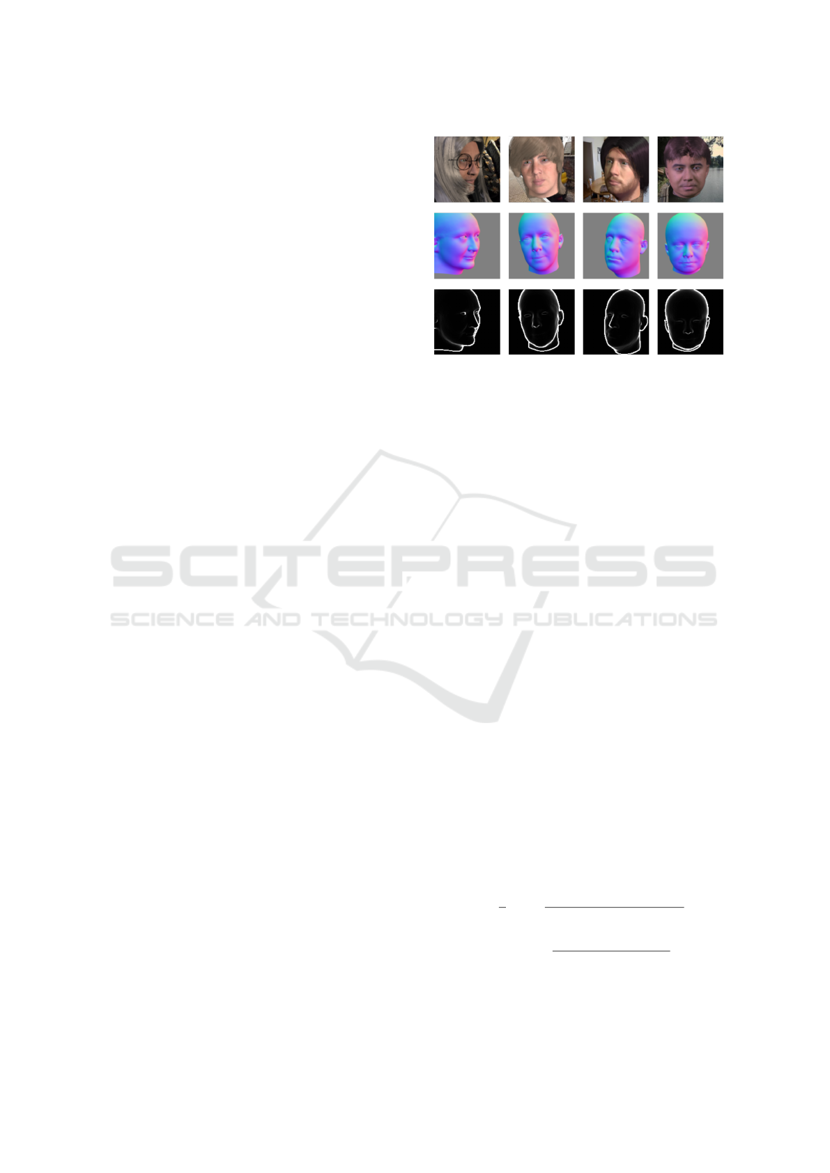
Figure 2: Training data samples. From top to bottom: Syn-
thetic facial images. Normal surface maps N. Gradient
Magnitude maps W .
and y is the corresponding coefficient vector shape.
Using this model, an infinite number of synthetic
faces can be generated by choosing a pair of param-
eters from a normal distribution y ∼ N(0,1). For
the hair we use different models from the (Hu et al.,
2015) data set with different colors and the Kajiya-
kay model (Kajiya and Kay, 1989) for the hair light-
ing rendering. We also use different male and female
face textures directly mapped with the 3D head model
and we align the head with a 3D eyes model where we
randomly change the color of the iris for each head
model. Finally, we also simulate six different 3D
glasses models to create some occlusions. Once the
different 3D components were aligned, random heads
are generated under various illumination conditions,
shadows, poses, scales, coefficients for physically-
based materials. Finally, to make the model insen-
sitive to the background, a random background image
taken from the COCO data set (Lin et al., 2014) is
added. Some examples of the training data set used
for this work are shown in Fig. 2.
Once the final 3D head model has been gener-
ated as detailed above, we compute the normal sur-
face only for the head and eyes models by using the
angle weighted method from (Klasing et al., 2009) as
written in (2). Normal values n
i
are calculated for
each vertex location p
i
∈ Re
3
, given the set of vertices
q
i,1
,q
i,2
,...,q
i,k
that are adjacent to p
i
.
n
i
=
1
k
k
∑
j=1
ω
j
[q
i, j
− p
i
] × [q
i, j+1
− p
i
]
|[q
i, j
− p
i
] × [q
i, j+1
− p
i
]|
,
ω
j
= arccos
hq
i, j
− p
i
,q
i, j+1
− p
i
i
|q
i, j
− p
i
||q
i, j+1
− p
i
|
.
(2)
The choice fell on the use of normals for various
reasons. First, components of normal field define lo-
VISAPP 2020 - 15th International Conference on Computer Vision Theory and Applications
362
cal geometric properties and hence disentangled from
one another across certain distances in the sense that
we can predict them completely independently, in
contrast to the depth values which should be predicted
all together. That is, without knowing the depth value
of the tip of the nose, for example, one cannot predict
the value for the eyes. Second, normals are invariant
to translation and scaling. To improve the quality of
3D reconstruction, the generation of gradient magni-
tude map |∇ f (x, y)| from the pixel-wise depth image
is proposed (third row in Fig. 2). The effect of using
this information is analysed in Section 3.3
3.2 Network Structure
The proposed GAN architecture is based on (Su et al.,
2018) work, where a network has been trained to map
the normal surface map from a sketch and a binary
point mask inputs. Some changes have been made
to this network to adapt it to our problematic (more
details in Fig. 3).
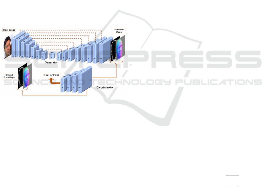
Figure 3: Our neural network architecture aims to gener-
ate two maps given facial input image. The input training
data as is shown on the left is composed of a facial input
image and two ground-truth maps: N and W. The encoder-
decoder’s input is the image of the face, while at the output
it produces two different maps (shown on the right). Af-
ter that, we inject ground truth and generated maps together
with the facial image as the input of discriminator. In this
stage, we check if the generated maps are real or fake, so
we encourage the encoder-decoder to produce more realis-
tic maps according to face image input. The spatial size and
the number of layers are indicated in and above each block,
respectively.
The model is composed of a encoder-decoder net-
work and a discriminator, proposed in (Ronneberger
et al., 2015). All training images have 128 × 128 pix-
els size. As an input, we stack three images, the facial
image (RGB), N (three channels) and W (single chan-
nel), while we have only two generated maps.
The encoder has the same elements as the discrim-
inator (discussed below), the decoder is composed of
ReLU activation function, deconvolution, batch nor-
malization, and a dropout unit. To reduce the informa-
tion loss between successive layers, we use a symmet-
ric connection between the encoder and the decoder
(Ronneberger et al., 2015). Therefore, we concate-
nate each layer of the encoder with the corresponding
channel in the decoder. The encoder-decoder is com-
posed of 16 layers. In the output layer, tanh is used as
an activation function, since N lies in the range [-1, 1].
The discriminator is composed of 4 layers, and it is
inspired by the encoder. Each layer is composed of:
convolution, batch normalization, and ReLU activa-
tion function. We adopt the loss function used in (Su
et al., 2018) for our purposes. Our objective function
becomes:
F = E
x∼p
data
,y∼p
m
[D(y/x)] − E
˜y∼p
gen
[D( ˜y/x)]−
λ
1
L
2
,
L
2
= E
y∼p
m
, ˜y∼p
gen
[||y − ˜y||
2
]
(3)
Where x represents the input face image, y is the
corresponding concatenated input maps, ˜y is the gen-
erated outputs. P
data
, P
m
, and P
gen
are the distributions
of real input data, input map and generated outputs
data, respectively. The encoder-decoder loss is mixed
with a pixel wised loss L
2
penalized by λ
1
to mea-
sure the difference between the generated maps and
the real input maps, and so to supervise the training
process.
3.3 3D Face Reconstruction
Our 3D reconstruction solution is based on the inte-
gration of normals guided by the magnitude of the
depth gradient, to improve the reconstruction preci-
sion in the presence of discontinuities. For this, we
retrieve the two output maps W and N from the gen-
erative model where:
• W : R
2
→ R is the magnitude of depth gradient,
• N : R
2
→ R
3
is the normal surface map.
Thenceforth, we compute depth gradient G based on
N as described in the following:
G : R
2
→ R
2
G(u,v) =
p(u,v)
q(u,v)
=
−
N
x
(u,v)
N
z
(u,v)
−
N
y
(u,v)
N
z
(u,v)
(4)
where N
x
, N
y
, and N
z
are the three components of N
and (u,v) represents the pixels of the discrete domain
Ω ⊂ R
2
. After that, we feed G(u, v) and W (u, v) into a
weighted least squares solver defined in a continuous
setting as follows:
argmin
h
ZZ
u,v∈Ω
w(u,v)||∇h(u,v) − G(u,v)||
2
dudv
(5)
Monocular 3D Head Reconstruction via Prediction and Integration of Normal Vector Field
363
w(u,v) =
1
1 + λW (u,v)
(6)
w(u,v) is the weight term used to enforce confor-
mity of the reconstructed surface with the gradient
term near the face discontinuities. In (6), λ is a crit-
ical parameter to tune (see details in section 4.2). In
this step, we estimate depth map values of a function
h : R
2
→ R within the reconstruction domain Ω where
G and W are defined. In the discrete setting, our min-
imization problem is formulated as below:
argmin
h
∑
u,v∈Ω
w
u+0.5,v
(h
u+1,v
− h
u,v
− p
u+0.5,v
)
2
+w
u,v+0.5
(h
u,v+1
− h
u,v
− q
u,v+0.5
)
2
(7)
Where (u + 0.5, v) and (u,v + 0.5) are the average
points between two successive pixels along the hor-
izontal and vertical axes respectively. For example,
gradient between pixels is defined in this way:
p
u+0.5,v
=
1
2
(p
u,v
+ p
u+1,v
)
q
u,v+0.5
=
1
2
(q
u,v
+ q
u,v+1
)
(8)
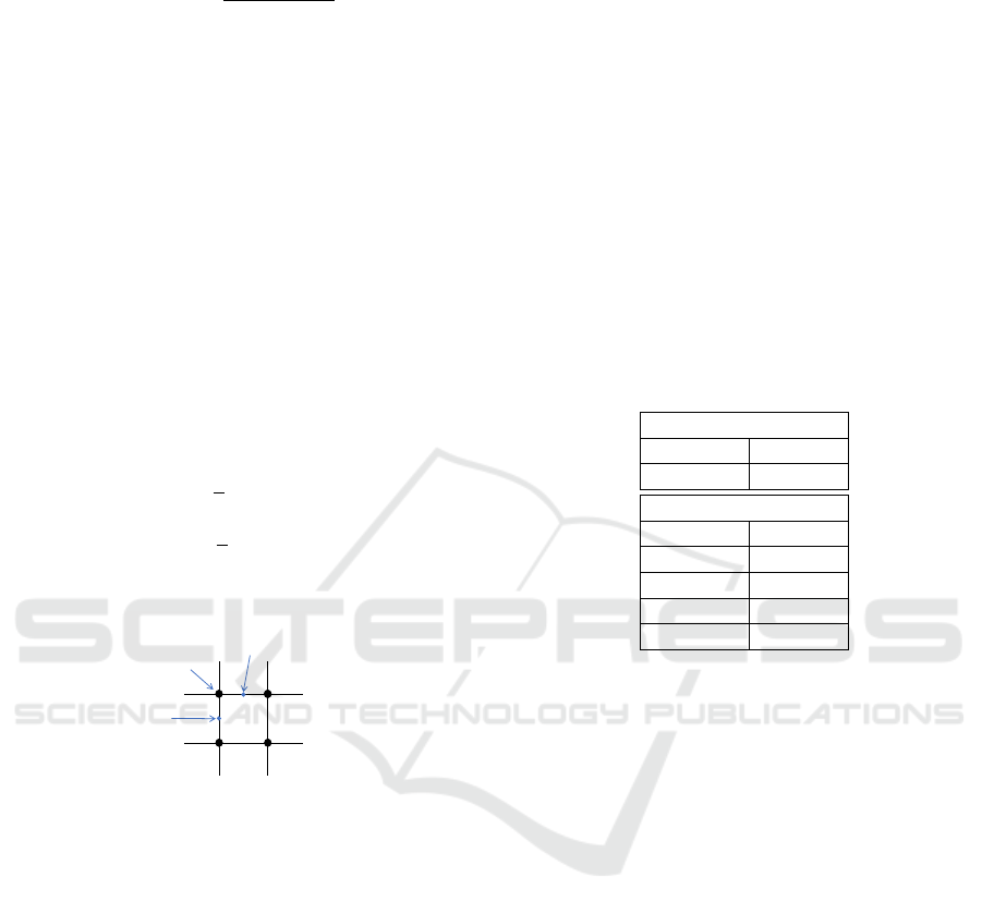
Figure 4: Illustration of our discretization method.
An illustration of our discretization method on a
regular square 2D grid is shown in Fig. 4. This is a
classical linear least-square problem, we solve it us-
ing the Ceres solver (Agarwal et al., ). Evaluation of
the reconstruction quality is given in section 4.2.
4 EXPERIMENTAL RESULTS
This section presents three sets of experiments that
were conducted to evaluate the performance of our 3D
reconstruction method. Firstly, we discuss the quality
of our training model in Section 4.1. Then, we show
our contribution to the reconstruction method and the
advantage it brings compared to other normals inte-
grations method in Section 4.2. Finally, we verify
this by qualitative and quantitative experiments on a
known database in Section 4.3.
Test Data set: To evaluate the quality of predicted
maps from our trained model and also our 3D recon-
struction method, we generate a test data set from
our generator described in the Section 3.1. This
test data set is used in our experiments. It consists
of 200 images of people (equitably distributed be-
tween males and females) generated with their corre-
sponding ground truth maps that include face images,
normal surface maps, gradient magnitude maps, and
depth maps. Depth is measured in units equivalent to
the pixel size.
4.1 Training Evaluation
Table 1: Mask and Normals evaluations for test data set. We
show in the top table part our segmentation results using
precision and recall percentage. The second part contains
angular error results.
Mask Evaluation
precision 93.72 %
recall 98.40 %
Normals Evaluation
Mean 10.01°
Std 12.45°
< 10° 67.50 %
< 20° 92.65 %
< 30° 97.13 %
To train the model, we have used 40,000 facial images
(20,000 for males and also for females) and their cor-
responding maps. We train the model for about 1700
epochs with a learning rate of 1e − 4, 64 as a batch
size, 500 for λ
1
, and using RMSprop optimizer. We
also add random blur effect and gaussian noise as data
augmentation.
To evaluate our Image-to-Image translation
model, we show in Fig. 5 different examples with
ground truth and maps produced by our GAN model.
We can well notice that with the use of our synthetic
data which contain occlusions (hair, glasses, random
backgrounds), the network succeeds to separate
properly the whole head. In situations where there
are covered parts, the network tries predicting a more
approximate form of the precise shape hidden by
the hair in most cases. Using the test database, we
performed some experiments to evaluate the accuracy
of our network. Table 1 shows the results indicating
a significant percentage of precision and recall,
which explains that most of the pixels produced by
the network correspond to the pixels of ground truth
maps. In a second time, we evaluated the precision
on the N maps and for this, we calculated the angular
error between the maps of the ground truth and those
produced by the network.
VISAPP 2020 - 15th International Conference on Computer Vision Theory and Applications
364
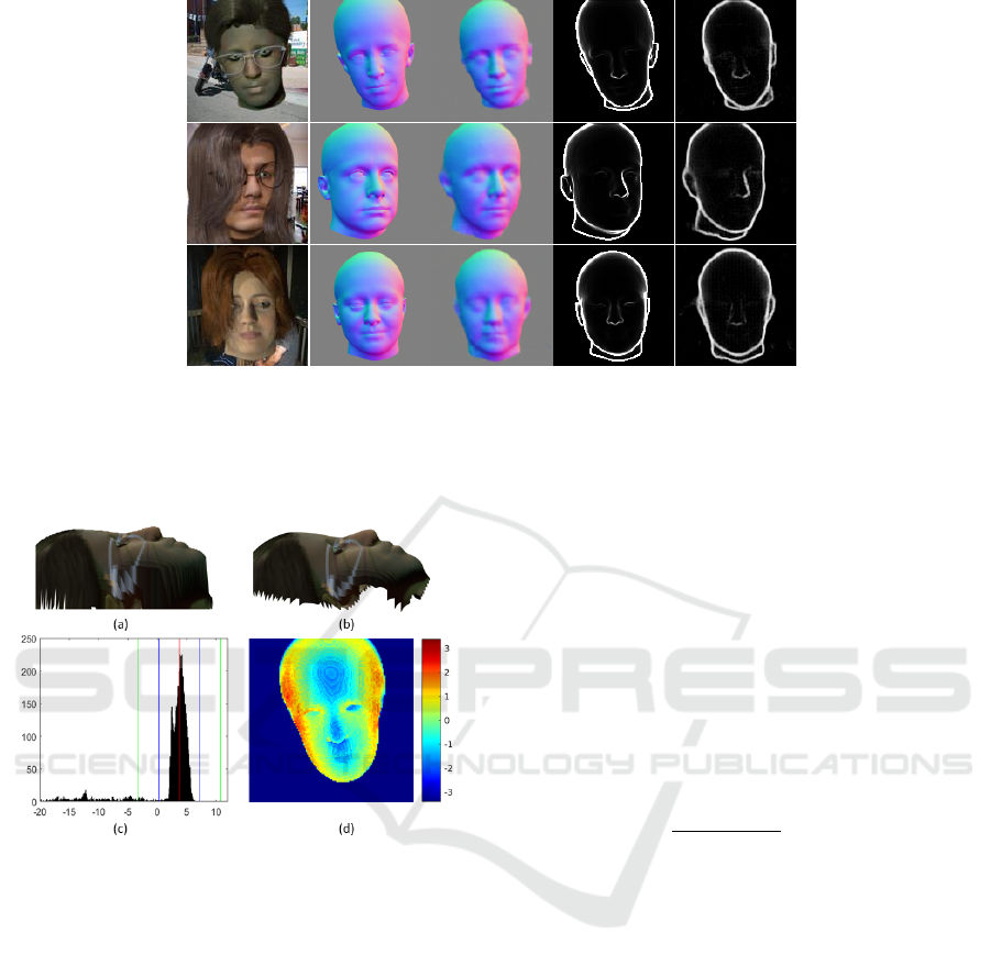
Figure 5: Comparison between ground-truth and estimates N and W maps. The first column contains the facial input image,
second and fourth columns contain ground-truth maps, third and fifth contain estimated maps.
4.2 Reconstruction Method Evaluation
Figure 6: Example of reconstruction result on synthetic data
from test data set
(a) Ground truth surface.
(b) Reconstructed surface.
(c) Histogram of residuals. Red, green and blue lines indi-
cate M
val
, M
val
± θ and M
val
± 3σ
M
respectively.
(d) Heat map with pixels errors after eliminating the bias.
The depth error is measured in units equivalent to pixels.
The image resolution is 128 × 128.
Using the test data set, we evaluate in this step, the
efficiency of our proposed method in 3D face recon-
struction. To do this, firstly we describe the λ param-
eter tuning procedure to optimize our reconstruction
method. Secondly, we show a comparison between
the ground truth and the reconstructed depth map us-
ing the optimal λ value that minimizes the reconstruc-
tion error. Once the depth is reconstructed, we com-
pare it to the ground truth, available in the test set.
The evaluation procedure used to find the optimal λ is
implemented as follows:
Step 1: compute the error map between the ground
truth and the reconstructed depth maps :
Err
M
= d
GT
− d
R
where z
GT
and z
R
are the ground truth and re-
constructed depths respectively; only the in-
tersection of domains Ω
GT
and Ω
R
is used.
Step 2: compute median value M of Err
M
and given
a fixed threshold θ = 7, we compute the stan-
dard deviation σ
M
of Err
M
for values which
lie in [M
val
− θ,M
val
+ θ].
Step 3: compute the variance V
i
of Err
M
in [M
val
−
3σ
M
,M
val
+ 3σ
M
] range.
We perform these steps for all test examples and we
compute σ =
q
∑
N
i=1
Var
i
/N for different λ values
ranging from 0 to 0.3. The influence of the choice
of λ on the 3D reconstruction is show in Fig. 8. The
choice λ = 0 corresponds to the least squares solution
without weighting. We found that the optimal value
is λ = 0.1. This value is used in all experiments here-
inafter. In Fig. 6, we illustrate an example from the
comparison procedure described above.
4.3 Final Evaluation
In order to analyze the performance of the pipeline as
a whole, we performed a qualitative experiment on a
set of images of celebrities and a quantitative experi-
ment on a 3D facial data set to test its accuracy.
For qualitative analysis, we show in Fig. 7 our re-
sults on the image of certain celebrities. One can see
that our method produces high-quality results that bet-
ter fit the overall structure. As we use a full 3DMM
head model that also includes the cranial part, our
method allows us to recover the 3D model of the head
Monocular 3D Head Reconstruction via Prediction and Integration of Normal Vector Field
365
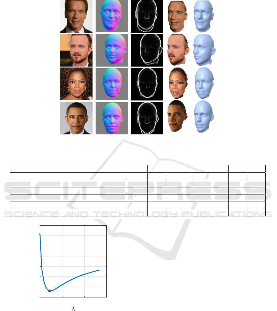
Figure 7: Visual surface reconstruction results from some celebrities facial images. Columns contain in order; input image,
estimated N map, estimated W map and the last two columns contain 3D shape reconstruction.
Table 2: Quantitative comparison on the BU-3DFE (Yin et al., 2006) data set. Lowers are better.
Method Mean Std Median 90% largest ¯e σ
(Kemelmacher-Shlizerman and Basri, 2010) 3.89 4.14 2.94 7.34 N/A N/A
(Zhu et al., 2015) 3.85 3.23 2.72 6.82 N/A N/A
(Richardson et al., 2017) 3.61 2.99 2.72 6.82 N/A N/A
(Sela et al., 2017) 3.51 2.69 2.65 6.59 N/A N/A
(Feng et al., 2018a) 2.78 2.04 1.73 5.30 N/A N/A
Ours 3.04 1.78 2.62 5.48 0.10 2.18
0 0.2 0.4 0.6
1.04
1.06
1.08
1.1
1.12
1.14
1.16
1.18
Std
Figure 8: The effect of λ on reconstruction accuracy in
terms of standard deviation on the test data set.
for any visible pixel on the image and it also predicts
any area hidden by the hair (third and fourth row in
Fig. 7). We also indicate the inferior quality of recon-
struction for surfaces containing the neck due to the
discontinuity between the face and neck parts (first
and second rows in Fig. 7).
Quantitative results are reported in Table 2. For
evaluation, we use the BU-3DFE (Yin et al., 2006)
data set which contains 3D faces of 100 subjects with
seven different expressions and each 3D model has
corresponding 2D images. Using only neutral ex-
pressions subjects for our comparison process, we
crop each reconstructed model on the part represent-
ing the valid pixels to take into account in the compar-
ison. After alignment and registration process based
on iterative closest point (ICP) with the ground truth
model, we compute the absolute depth error. Note
that we eliminate examples when the alignment pro-
cess fails. Finally, we report depth errors evaluated
by mean, standard deviation, median, and the aver-
age ninety percent most significant error. Note that
we report the results obtained on the same data set di-
rectly from (Feng et al., 2018a) paper. From Table 2,
we can see that our method produces results compa-
rable to the state of the art. The performance of (Feng
et al., 2018a) work is slightly better than ours, and
we believe that is due to the fact they use part of the
BU-3DFE (Yin et al., 2006) data set for training. This
data set is acquired using a special sensor, while our
model is trained only with generated synthetic data.
VISAPP 2020 - 15th International Conference on Computer Vision Theory and Applications
366
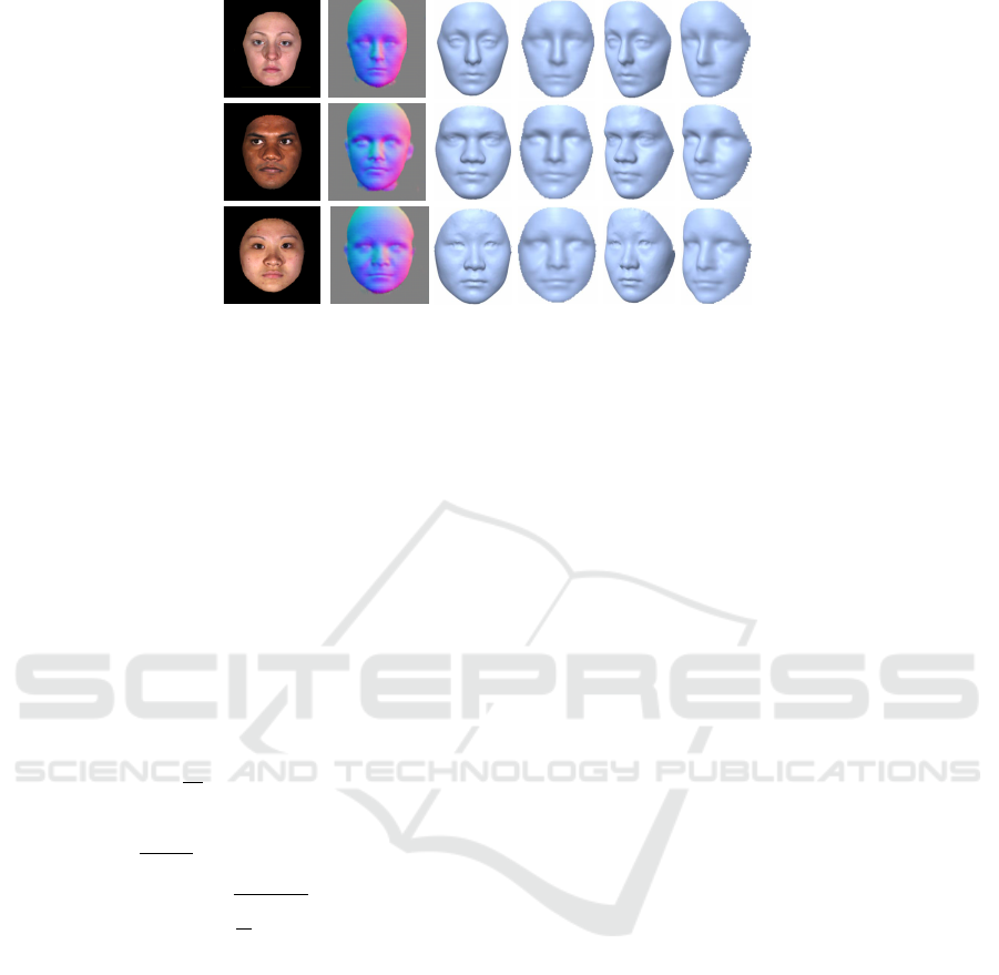
Figure 9: Reconstruction results for three BU-3DFE examples from two different viewpoints. From left to right: input
image, normal map (N), front-view ground-truth model, front-view reconstructed model, slide-view ground-truth model and
side-view reconstructed model.
We also provide another way of estimating the er-
ror between the reconstruction and the ground truth.
The criterion is standard deviation σ of per-vertex er-
rors between the reconstruction and the ground truth
projected on the normals of the ground truth (mean of
this error being very close to zero after surface regis-
tration). By doing so we evaluate the error between
two surfaces in the normal direction instead of dis-
tances between points. Since the models do not have
the same meshes, we find nearest neighbor for each
vertex of the reconstruction. The criteria are defined
as follows:
¯e =
1
M
M
∑
k=1
(a
k
− b
k
)n
i
V =
1
M − 1
M
∑
k=1
((a
k
− b
k
)n
i
− ¯e)
2
σ =
s
1
N
E
∑
k=1
V
k
(9)
where N is the total number of examples in the BU-
3DFE (Yin et al., 2006) data set, M is the total number
of vertices per model. a
k
and b
k
are the coordinates of
vertices from the estimated and ground truth models
respectively and n
i
is the normals coordinates from
the ground truth model. The values of this calculation
are reported in the sixth and seventh column of the
Table 2.
5 CONCLUSION
In this work, we have presented a hybrid 3D face re-
construction approach composed of both learning and
geometric based methods. The first stage of our main
block is an image-to-image translation network that
produces normal surface map (N) and gradient mag-
nitude map (W ) from a facial input image. The sec-
ond stage is integration of normals based on weighted
least squares, which uses our network outputs to gen-
erate the depth facial map. Our deep learning model
has been trained on a fully synthetic facial data set.
We have performed three experiments to evalu-
ate our pipeline performance: first, we show that the
neural network generates accurate maps of normals.
Next, experiments confirm the effectiveness of using
the W map as a weight during the reconstruction step
to resolve discontinuous boundary artifacts. In the
final experiment, we demonstrate that the proposed
framework achieves the state-of-the-art performance
in 3D face reconstruction. We also propose a new
error calculation method, which, we think, is more
representative for this type of evaluation. Using this
criterion with explicitly written equations avoids any
ambiguity on how exactly the evaluation is done and
what is the meaning of the obtained value.
Two loss functions L
1
and L
2
have been tested as
a pixel loss for network training. L
2
shows a bet-
ter performance in fine detail reconstruction. And
yet some facial features of generated normal maps
are still slightly blurred. One possible improvement
would be to increase the network complexity and to
modify the output layers in order to get sharp details.
Despite the robust performance in many cases, our
method has a certain number of limitations. The head
generator does not include facial expressions and has
limited age range. But these limitations can be over-
come by using a better synthetic data generator, it is
not a fundamental limitation of the proposed method.
Furthermore this method is generic and can be ap-
plied to any kind of 3D object reconstruction if the
right data generator is available. Synthetic data sets
allow us to train complex models with virtually un-
limited data supply. It accelerates training process by
Monocular 3D Head Reconstruction via Prediction and Integration of Normal Vector Field
367

drastically reducing data markup step. On the other
hand synthetic data can introduce certain biases in the
learning process and therefore one should try to make
the generator as photo-realistic as possible. One way
of doing that is using GAN architectures in combina-
tion of classical 3D rendering.
REFERENCES
Abate, A. F., Nappi, M., Riccio, D., and Sabatino, G.
(2007). 2d and 3d face recognition: A survey. Pat-
tern Recognition Letters, 28(14):1885–1906.
Agarwal, S., Mierle, K., and Others. Ceres solver. http:
//ceres-solver.org.
Agrawal, A., Raskar, R., and Chellappa, R. (2006). What
is the range of surface reconstructions from a gradient
field? In European conference on computer vision,
pages 578–591. Springer.
Amberg, B., Knothe, R., and Vetter, T. (2008). Expres-
sion invariant 3d face recognition with a morphable
model. In Automatic Face & Gesture Recognition,
2008. FG’08. 8th IEEE International Conference on,
pages 1–6. IEEE.
Bansal, A., Russell, B., and Gupta, A. (2016). Marr revis-
ited: 2d-3d alignment via surface normal prediction.
In Proceedings of the IEEE conference on computer
vision and pattern recognition, pages 5965–5974.
Bas, A., Smith, W. A., Bolkart, T., and Wuhrer, S. (2016).
Fitting a 3d morphable model to edges: A comparison
between hard and soft correspondences. In Asian Con-
ference on Computer Vision, pages 377–391. Springer.
Blanz, V. and Vetter, T. (1999). A morphable model for
the synthesis of 3d faces. In Proceedings of the 26th
annual conference on Computer graphics and interac-
tive techniques, pages 187–194. ACM Press/Addison-
Wesley Publishing Co.
Blanz, V. and Vetter, T. (2003). Face recognition based
on fitting a 3d morphable model. IEEE Transac-
tions on pattern analysis and machine intelligence,
25(9):1063–1074.
Booth, J., Antonakos, E., Ploumpis, S., Trigeorgis, G.,
Panagakis, Y., Zafeiriou, S., et al. (2017). 3d face
morphable models in-the-wild. In Proceedings of
the IEEE Conference on ComputerVision and Pattern
Recognition.
Dai, H., Pears, N., Smith, W. A. P., and Duncan, C. (2017).
A 3d morphable model of craniofacial shape and tex-
ture variation. In The IEEE International Conference
on Computer Vision (ICCV).
Dou, P., Shah, S. K., and Kakadiaris, I. A. (2017). End-to-
end 3d face reconstruction with deep neural networks.
In Proc. IEEE Conference on Computer Vision and
Pattern Recognition, pages 21–26.
Feng, M., Zulqarnain Gilani, S., Wang, Y., and Mian, A.
(2018a). 3d face reconstruction from light field im-
ages: A model-free approach. In Proceedings of the
European Conference on Computer Vision (ECCV),
pages 501–518.
Feng, Y., Wu, F., Shao, X., Wang, Y., and Zhou, X.
(2018b). Joint 3d face reconstruction and dense align-
ment with position map regression network. arXiv
preprint arXiv:1803.07835.
Frankot, R. T. and Chellappa, R. (1988a). A method
for enforcing integrability in shape from shading al-
gorithms. IEEE Trans. Pattern Anal. Mach. Intell.,
10(4):439–451.
Frankot, R. T. and Chellappa, R. (1988b). A method for
enforcing integrability in shape from shading algo-
rithms. IEEE Transactions on pattern analysis and
machine intelligence, 10(4):439–451.
Furukawa, Y. and Ponce, J. (2009). Accurate camera cali-
bration from multi-view stereo and bundle adjustment.
International Journal of Computer Vision, 84(3):257–
268.
Ghosh, A., Fyffe, G., Tunwattanapong, B., Busch, J., Yu,
X., and Debevec, P. (2011). Multiview face capture
using polarized spherical gradient illumination. In
ACM Transactions on Graphics (TOG), volume 30,
page 129. ACM.
Gonzalez-Mora, J., De la Torre, F., Guil, N., and Zapata,
E. L. (2010). Learning a generic 3d face model from
2d image databases using incremental structure-from-
motion. Image and Vision Computing, 28(7):1117–
1129.
Han, X., Ugail, H., and Palmer, I. (2009). Gender classifica-
tion based on 3d face geometry features using svm. In
CyberWorlds, 2009. CW’09. International Conference
on, pages 114–118. IEEE.
Harker, M. and Oleary, P. (2015). Regularized recon-
struction of a surface from its measured gradient
field. Journal of Mathematical Imaging and Vision,
51(1):46–70.
Hsieh, J.-W., Liao, H.-Y. M., Ko, M.-T., and Fan, K.-C.
(1995). Wavelet-based shape from shading. Graphical
Models and Image Processing, 57(4):343–362.
Hu, L., Ma, C., Luo, L., and Li, H. (2015). Single-view
hair modeling using a hairstyle database. ACM Trans-
actions on Graphics (Proceedings SIGGRAPH 2015),
34(4).
Huber, P., Feng, Z.-H., Christmas, W., Kittler, J., and
Ratsch, M. (2015). Fitting 3d morphable face mod-
els using local features. In Image Processing (ICIP),
2015 IEEE International Conference on, pages 1195–
1199. IEEE.
Hudon, M., Grogan, M., Pag
´
es, R., and Smoli
´
c, A. (2018).
Deep normal estimation for automatic shading of
hand-drawn characters. In European Conference on
Computer Vision, pages 246–262. Springer.
Kajiya, J. T. and Kay, T. L. (1989). Rendering fur with
three dimensional textures. In ACM Siggraph Com-
puter Graphics, volume 23, pages 271–280. ACM.
Karac¸alı, B. and Snyder, W. (2003). Reconstructing dis-
continuous surfaces from a given gradient field using
partial integrability. Computer Vision and Image Un-
derstanding, 92(1):78–111.
Kemelmacher-Shlizerman, I. and Basri, R. (2010). 3d face
reconstruction from a single image using a single ref-
VISAPP 2020 - 15th International Conference on Computer Vision Theory and Applications
368

erence face shape. IEEE transactions on pattern anal-
ysis and machine intelligence, 33(2):394–405.
Klasing, K., Althoff, D., Wollherr, D., and Buss, M. (2009).
Comparison of surface normal estimation methods for
range sensing applications. In 2009 IEEE Interna-
tional Conference on Robotics and Automation, pages
3206–3211. IEEE.
Kovesi, P. (2005). Shapelets correlated with surface nor-
mals produce surfaces. In Tenth IEEE International
Conference on Computer Vision (ICCV’05) Volume 1,
volume 2, pages 994–1001. IEEE.
Lin, T.-Y., Maire, M., Belongie, S., Hays, J., Perona, P.,
Ramanan, D., Doll
´
ar, P., and Zitnick, C. L. (2014).
Microsoft coco: Common objects in context. In Euro-
pean conference on computer vision, pages 740–755.
Springer.
Lun, Z., Gadelha, M., Kalogerakis, E., Maji, S., and Wang,
R. (2017). 3d shape reconstruction from sketches via
multi-view convolutional networks. In 2017 Interna-
tional Conference on 3D Vision (3DV), pages 67–77.
IEEE.
Qiu, J., Cui, Z., Zhang, Y., Zhang, X., Liu, S., Zeng, B., and
Pollefeys, M. (2019). Deeplidar: Deep surface normal
guided depth prediction for outdoor scene from sparse
lidar data and single color image. In Proceedings of
the IEEE Conference on Computer Vision and Pattern
Recognition, pages 3313–3322.
Qu
´
eau, Y. and Durou, J.-D. (2015). Edge-preserving inte-
gration of a normal field: Weighted least-squares, tv
and lˆ 1 approaches. In International Conference on
Scale Space and Variational Methods in Computer Vi-
sion, pages 576–588. Springer.
Qu
´
eau, Y., Durou, J.-D., and Aujol, J.-F. (2018). Normal in-
tegration: a survey. Journal of Mathematical Imaging
and Vision, 60(4):576–593.
Richardson, E., Sela, M., Or-El, R., and Kimmel, R.
(2017). Learning detailed face reconstruction from a
single image. In Proceedings of the IEEE Conference
on Computer Vision and Pattern Recognition, pages
1259–1268.
Ronneberger, O., Fischer, P., and Brox, T. (2015). U-net:
Convolutional networks for biomedical image seg-
mentation. In International Conference on Medical
image computing and computer-assisted intervention,
pages 234–241. Springer.
Sela, M., Richardson, E., and Kimmel, R. (2017). Unre-
stricted facial geometry reconstruction using image-
to-image translation. arxiv.
Simchony, T., Chellappa, R., and Shao, M. (1990). Di-
rect analytical methods for solving poisson equations
in computer vision problems. IEEE transactions on
pattern analysis and machine intelligence, 12(5):435–
446.
Su, W., Du, D., Yang, X., Zhou, S., and Fu, H. (2018). Inter-
active sketch-based normal map generation with deep
neural networks. Proceedings of the ACM on Com-
puter Graphics and Interactive Techniques, 1(1):22.
Sumner, R. W., Schmid, J., and Pauly, M. (2007). Em-
bedded deformation for shape manipulation. In ACM
Transactions on Graphics (TOG), volume 26, page 80.
ACM.
Terzopoulos, D. (1988). The computation of visible-surface
representations. IEEE Transactions on Pattern Analy-
sis & Machine Intelligence, (4):417–438.
Thies, J., Zollhofer, M., Stamminger, M., Theobalt, C., and
Nießner, M. (2016). Face2face: Real-time face cap-
ture and reenactment of rgb videos. In Proceedings of
the IEEE Conference on Computer Vision and Pattern
Recognition, pages 2387–2395.
Tran, A. T., Hassner, T., Masi, I., and Medioni, G. (2017).
Regressing robust and discriminative 3d morphable
models with a very deep neural network. In Computer
Vision and Pattern Recognition (CVPR), 2017 IEEE
Conference on, pages 1493–1502. IEEE.
Trigeorgis, G., Snape, P., Zafeiriou, S., and Kokkinos, I.
(2017). Normal Estimation For ”in-the-wild” Faces
Using Fully Convolutional Networks. In Computer
Vision and Pattern Recognition (CVPR).
Wang, X., Fouhey, D., and Gupta, A. (2015). Designing
deep networks for surface normal estimation. In Pro-
ceedings of the IEEE Conference on Computer Vision
and Pattern Recognition, pages 539–547.
Wang, Y., Bu, J., Li, N., Song, M., and Tan, P. (2012). De-
tecting discontinuities for surface reconstruction. In
Proceedings of the 21st International Conference on
Pattern Recognition (ICPR2012), pages 2108–2111.
IEEE.
Xie, W., Wang, M., Wei, M., Jiang, J., and Qin, J. (2019).
Surface reconstruction from normals: A robust dgp-
based disconti-nuity preservation approach. In Pro-
ceedings of the IEEE Conference on Computer Vision
and Pat-tern Recognition, pages 5328–5336.
Yin, L., Wei, X., Sun, Y., Wang, J., and Rosato, M. J.
(2006). A 3d facial expression database for facial
behavior research. In 7th international conference
on automatic face and gesture recognition (FGR06),
pages 211–216. IEEE.
Zhu, X., Lei, Z., Yan, J., Yi, D., and Li, S. Z. (2015). High-
fidelity pose and expression normalization for face
recognition in the wild. In Proceedings of the IEEE
Conference on Computer Vision and Pattern Recogni-
tion, pages 787–796.
Zollh
¨
ofer, M., Martinek, M., Greiner, G., Stamminger, M.,
and S
¨
ußmuth, J. (2011). Automatic reconstruction of
personalized avatars from 3d face scans. Computer
Animation and Virtual Worlds, 22(2-3):195–202.
Monocular 3D Head Reconstruction via Prediction and Integration of Normal Vector Field
369
