Left Ventricle Computational Model based on Patients

Three-dimensional MRI

Maria Narciso

1 a

, Ana Isabel Sousa

1 b

, Fernando Crivellaro

1 c

, Rui Valente de Almeida

1 d

Ant

onio Ferreira

2 e

and Pedro Vieira

1 f

FCT Nova, Caparica, Portugal

Cardiology Department, Hospital de Santa Cruz, Centro Hospitalar Lisboa Ocidental, Lisbon, Portugal

Keywords:

Heart Computational Model, Parallel Simulation, Cardiac Electrophysiology, Arrhythmia, CHASTE,

MATLAB, Virtual Heart.

Abstract:

The propagation of electric signal in the heart is bonded to the cardiac muscle (myocardium) geometry and

condition. In this regard we aim to build a patient-speciﬁc computational model of the myocardium based on

noninvasive imaging, with the long-term goal of being used to run simulations in electrophysiology studies.

Three-dimensional (3D) Magnetic Resonance Images (MRI) were processed using MATLAB



to build a

volumetric mesh which embodies the Left Ventricle (LV) and can later be read by third party applications.

This feature was tested with the open source software CHASTE (Cancer, Heart and Soft Tissue Environment)

to solve and visualize the propagation of an excitation wave.

Furthermore, an algorithm was developed capable of deﬁning the ﬁbre orientation for the resulting mesh, based

on the geometry described in literature. This experiment substantiates the expectation that parallel computing

simulations of the heart maybe used, in the near future, as a monitoring and diagnostic tool for the assessment

of cardiac arrhythmias in clinical practice.

1 INTRODUCTION

The work here described is part of a project cur-

rently being developed in collaboration with Hospi-

tal de Santa Cruz (Carnaxide, Portugal), where Physi-

cians and Techs contribute with not only datasets but,

above all, guidance and expertise. The ultimate goal

is to create an arrhythmia risk-stratiﬁcation tool using

noninvasive imaging as input. In order to accomplish

this, it is fundamental to develop a method capable of

assembling a 3D model of the heart, more speciﬁcally

of the LV, from the imaging datasets. This paper will

be focused on this very ﬁrst step of the process.

Cardiac electric impulses begin at the sinoatrial

node (natural pacemaker) and spread through the my-

ocytes, cardiac cells with membranes selectively per-

meable to K, Na and Ca ions. The movement of these

https://orcid.org/0000-0001-5079-9381

https://orcid.org/0000-0003-2980-4742

https://orcid.org/0000-0002-7534-9149

https://orcid.org/0000-0002-2269-7094

https://orcid.org/0000-0002-1623-7382

https://orcid.org/0000-0002-3823-1184

ions in and out of the intracellular space causes the po-

tential difference responsible for driving the electrical

signals to the contractile myocytes (Tse, 2016)(Di Yu

et al., 2014).

The heart walls that enclose the four cardiac

chambers are formed by myocardium, the muscular

tissue responsible for the heart contraction. The in-

ner part of the myocardium is called endocardium,

while the outermost part is usually called epicardium.

Most of the ventricular arrhythmias are the result of

some form of structural heart disease that causes the

myocardial tissue to become heterogeneous in terms

of electric conduction. Since most of the clinically

signiﬁcant ventricular arrhythmias arise from the LV,

and in order to simplify the model and reduce compu-

tational costs, we limited our analysis to this ventricle.

Cardiac magnetic resonance has started to re-

place ultrasound-based echocardiograms as the imag-

ing standard in clinical arrhythmology and electro-

physiology studies (De Maria et al., 2017). Beside

the advantage of being non-invasive while not us-

ing ionizing radiation. MRI provides excellent con-

trast between soft tissues, offering structural and func-

tional information. The images are computational re-

156

Narciso, M., Sousa, A., Crivellaro, F., Valente de Almeida, R., Ferreira, A. and Vieira, P.

Left Ventricle Computational Model based on Patients Three-dimensional MRI.

DOI: 10.5220/0008961601560163

In Proceedings of the 13th International Joint Conference on Biomedical Engineering Systems and Technologies (BIOSTEC 2020) - Volume 2: BIOIMAGING, pages 156-163

ISBN: 978-989-758-398-8; ISSN: 2184-4305

constructions of the signal received from sensors that

measure the particles resonance when cut off from an

excitation pulse of radio waves. Although this tech-

nology alone is not capable of detecting ﬁbres and

micro structures, the anatomical features extracted

from the resulting images provide the most advan-

tageous baseline to achieve in silico patient-speciﬁc

heart models. (Auricchio, Angelo, Singh, Jagmeet,

Rademakers, 2012). For this reason, this was the

imaging modality chosen as outset of our project.

Technical details of the method that has proven

to be able to generate three-dimensional models from

these images are described in the next chapter. Image

processing was done in MATLAB and the ﬁbre ori-

entation estimation code was written in Python. The

diagram in ﬁgure 1 despicts the overall workﬂow.

3D MRI

Myocardium segmentation

Fibers

orientation

STL

Other formats

Simulations

Figure 1: Workﬂow of the three-dimensional model assem-

bling process.

2 DEVELOPMENT OF THE

VENTRICLE MODEL

This section reports the methods used for develop-

ing the 3D computational model of the LV, built from

magnetic resonance images of a speciﬁc patient. The

methods described were designed in MATLAB 2015

and trusted to be broad enough to be used with most

patients, aside from subjects with severe cardiac de-

formities, as these cases are not standardized and

would require specially designed tools. The result is a

Stereolithography (STL) ﬁle representing the cardiac

muscle, which may later be opened and modiﬁed by

several applications.

2.1 Dataset

Ant

onio Ferreira provided anonymized images in DI-

COM format from a contrast-enhanced 3D cardiac

MRI exam that was considered to be entirely normal.

Any areas of myocardial ﬁbrosis would be visible in

the images as brighter areas amidst the darker cardiac

muscle. Therefore our process started from an ideal

case with homogeneous myocardial tissue.

The encoded images are made of voxels, the basic

element of a 3D image, in the same manner the pixel

is in 2D images. A voxel has three dimensions there-

fore it is referenced in space by three coordinates, its

intensity value can be in several different ranges as

the scales are not standardized.

In this acquisition, the whole slab is encoded re-

sulting in 3D image with high spatial resolution - size

of an individual voxel - and high signal-to-noise ratio.

The voxels are nearly isotropic, allowing reconstruc-

tion in any direction.

2.2 Segmentation of MR Data Set

From now on, the ﬁrst dimension elements of any 3D

matrix will be referred to as rows (along yy), the sec-

ond columns (along xx) and the third slices (along zz).

Information as voxel size, number of rows and

columns of each image, was obtained from the DI-

COM ﬁle info section and stored with the purpose

of being accessed along the process. The images,

which represent axial slices of the torso, were read to

a three-dimensional matrix with the dimensions rows

x columns x number of images, meaning they were

turned into two dimensional matrices stacked along

the z axis. The intensity values of every image are di-

vided by the maximum value of intensity, to obtain a

range from 0(lightest) to 1 (darkest), therefore the rest

of the transformations can be applied in any set inde-

pendently of the scale used in the exam, as of today

there is still not a standard range.

Our aim was not to develop an algorithm capable

of automatically segment the myocardium but to de-

velop semi-automatic tools to do so, as in this context

it was required that a physician guided and supervised

the entire process.

The ﬁrst required transformation is the rotation

of the matrix in order to attain the short-axis (SAX)

view. In this view, slices are perpendicular to the

long-axis (LAX) of the LV which allows us to exam-

ine cross-sections of both ventricles, where the cham-

bers walls are clearly distinguishable and the left ven-

tricle sections are usually annular.

Heart orientation and consequently the left ventri-

cle alignment, differs between individuals. On this

account and following the traditional cardiologist ap-

proach, we chose to navigate trough the different per-

spectives using cutting planes, illustrated by lines the

user deﬁnes.

As the licensed version of Matlab we had avail-

able did not support the imrotate3d function - which

allows the rotation of three dimensional objects in any

Left Ventricle Computational Model based on Patients Three-dimensional MRI

157

direction at any angle - we deﬁned a function which

rotates each slice (two dimensional rotation) around

its centre, the same number of degrees the drawn line

makes with the vertical axis. Next the whole matrix is

rotated 90

clockwise around the y axis, as the func-

tion rot90 is available in this version of the software

and allows the use of angles multiples of 90

. The

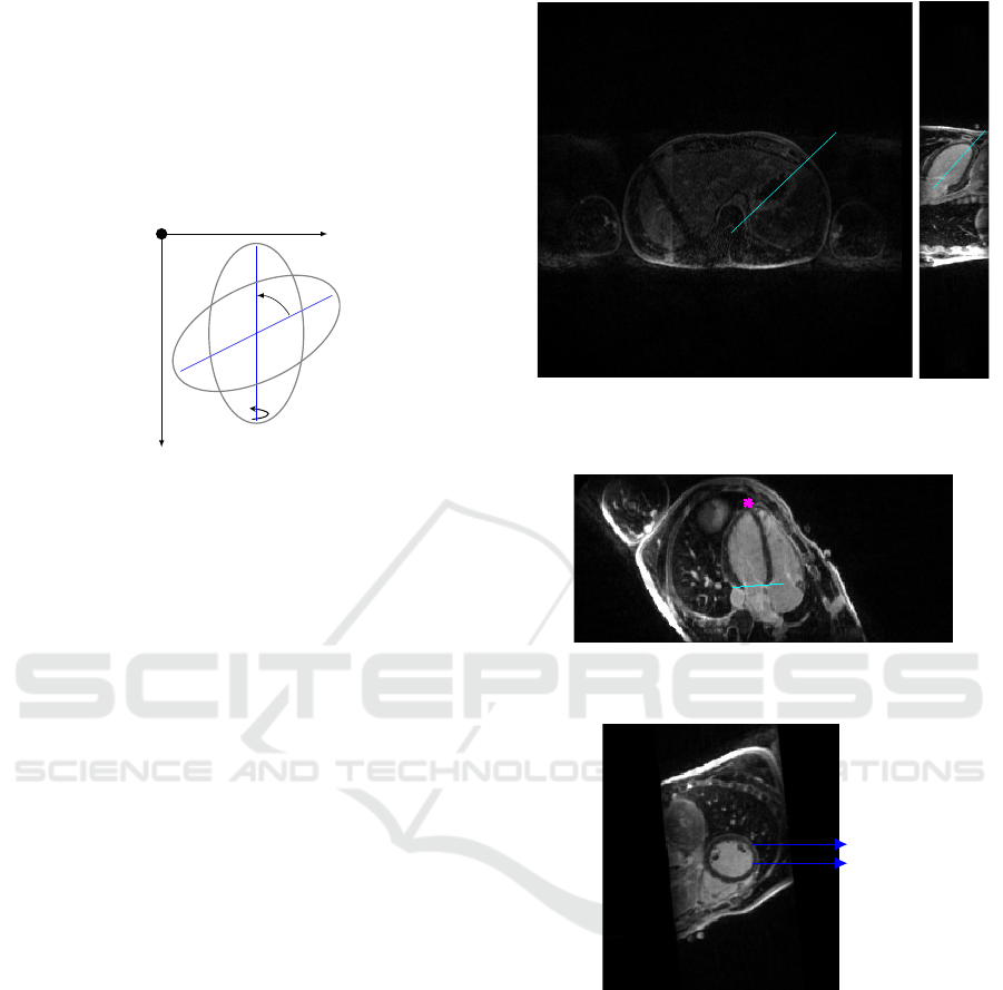
logic of the cutting plan is exempliﬁed in ﬁgure 2.

Figure 2: Rotation of 2D images based on the drawn lines,

ﬁrst in the amplitude of θ around the z axis and then 90

around the y axis.

For each transformation triggered by a line, two

new matrices are created, ﬁrst a copy of the origi-

nal, with the same size but with each slice rotated and

cropped, and with the second transformation another

copy with the ﬁrst and third dimensions permuted.

Starting from the axial view, the ﬁrst line must be

parallel to the inter-ventricular septum, right picture

of ﬁgure 3, the rotation results in the vertical long axis

view shown in the left picture of 3. Then one should

draw a bisecting line from the LV apex to the mitral

valve, this leads to the horizontal long axis view. The

user is then asked to mark the LV ventricle apex with

a point and the base with a line, ﬁgure 4, ﬁnally we

are presented with the SAX view. This cut generates

a matrix with the dimensions number of rows of each

image x columns x number of slices from base to apex.

An example of a slice from this object is shown in

ﬁgure 5.

Inside the LV chamber, the pixels represent blood

therefore the intensity levels are lower than that at the

pixels representing tissue. A point in this area and an-

other one at the myocardium outside border are man-

ually marked.

The grayconnected function is applied to select

the contiguous regions with similar intensities for

both points. The output is a binary image where

the pixels that are part of the region have the value

one. The two resulting areas enclose every pixel

with values between seedvalue-tolerance and seed-

value+tolerance. For the area inside the chamber

seedvalue is the pixel intensity level at the selected

point and the tolerance is a quarter of the difference

between this value and the intensity value at the sec-

Figure 3: Right: Axial view of the torso with a line drawn

parallel to the septum. Left: LAX vertical view with the

bisetrix line.

Figure 4: Horizontal LAX view with the apex marked in

pink and base of LV in cyan.

Pericardium

Myocardium

Figure 5: SAX view where both ventricles are visible.

ond point, hence adding only pixels with values closer

to the blood intensity than to the muscle. The shape

centre of mass is calculated and stored. The second

region is the actual segmented myocardium, gener-

ated following the same logic. There is a thin pro-

tetive layer surrounding the whole heart named peri-

cardium , ﬁgure 5. Because it is almost white, its pix-

els are beyond the intensity threshold and will not be

aggregated, however this layer is so thin that some-

times is borders are not distinguishable, therefore the

distance between the centre of mass is set as the maxi-

mum distance the value of the pixels above this radius

are change to zero. The result is a black and white im-

BIOIMAGING 2020 - 7th International Conference on Bioimaging

158

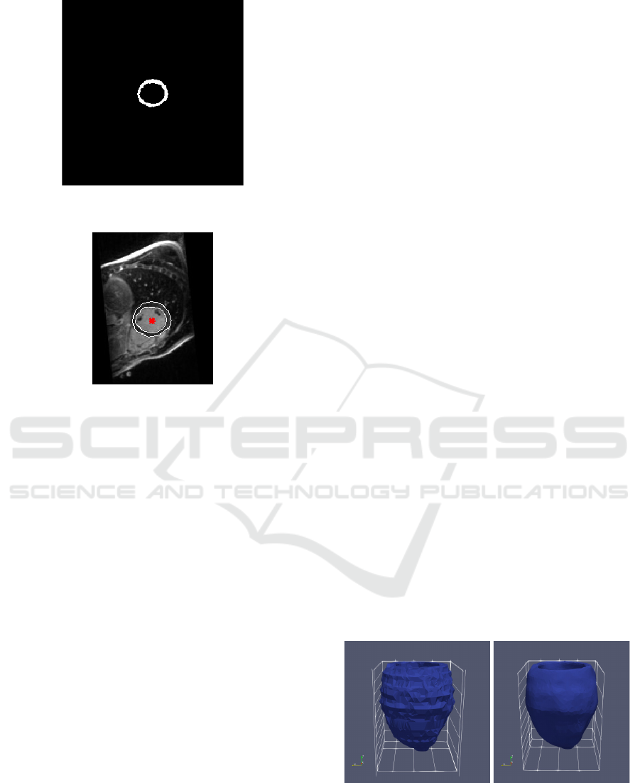
Figure 6: Binary image of the LV myocardium segmented

from the SAX slice

Figure 7: SAX view with the myocardium borders con-

toured in white and the centre of mass marked with a red

cross.

age representing a slice of the myocardium, ﬁgure 6,

its contours are shown in ﬁgure 7 on top of the origi-

nal slice.

The process above is repeated for every slice, the

ones representing the apex myocardium is visible as

a small circle, instead of a annulus, therefore only the

second point is needed. Each resulting image is saved

into a matrix with the same size as the last one created,

stacking the cross sections of the ventricle along the

third dimension.

2.3 3D Model and Formatting

At this stage the object is represented in a regular grid

in 3D space, thus the location of each voxel is de-

scribed by discrete values of row, column and page, to

get the real spacial coordinates the ﬁnd function was

called, as it returns the indexes of each voxel with a

value not zero and the respective coordinates where

saved in a matrix [r,c,p], then each element was mul-

tiplied by the voxel size for the respective dimension.

This transformation was applied at this stage and not

later for the simplicity of working with only point co-

ordinates. Regardless, this is a crucial step consider-

ing that, although STL structures are dimensionless

and the ﬁles contain no scale information, the output

must be ready to be handled by applications where

distances and dimensions matter.

It is possible to increase the resolution, multiply-

ing the number of points. Using linspace to generate

a vector with the size of each dimension, changing

the spacing from one to the desired integer number.

two meshgrids are generated one from the new vec-

tors and one from three vectors with the original spac-

ing. Then using bilinear interpolation with interpn, a

new matrix is created interpolating the original mesh-

grid with the new one. Higher resolution does not af-

fect the results, however, during the simulations, the

signal propagation can be observed with more detail,

as the mesh will be made of smaller blocks. As ex-

pected, this comes with a high computational price.

The function alphashape creates a surface around

all the deﬁned points, using the variable alpha to de-

ﬁne the tightness, the user deﬁnes the optimal alpha

value so that the chamber is open while the walls are

closed. Next, boundaryFacets is called to get the tri-

angles faces and each concerning vertex that form the

surfaces of the volume, this process is known as tes-

sellation, ﬁlling a surface with geometric shapes (in

this case triangles) without overlapping or forming

gaps). smoothpatch (Kroon, 2010) was applied to

polish the rough edges, this function takes each ver-

tex, checks the neighbours from the same facet and

moves them in a way that the distance between them

becomes more uniform, keeping the number of trian-

gles.

The last step in MATLAB is the exportation to a

STL ﬁle, supported by many software and applica-

tions.

The stlwrite (Holcombe, 2011) function was used

to export the triangulated structure to a ﬁle with the

standardized format. Both the smoothed model and

the one from the previous step are exported, so they

can be tested against each other, ensuring that this aes-

thetic alterations do not compromise the model. A

comparison of both can be found in ﬁgure 8.

2828

3030

Y AxisY Axis

3232

3434

X AxisX Axis

28283030

Y AxisY Axis

32323434

2222

4444

Z AxisZ Axis

1010

2424

3434 3232

Y AxisY Axis

3030

3030 3030

X AxisX Axis

3434 3232

Y AxisY Axis

X AxisX Axis

3030

Z AxisZ Axis

1010

Figure 8: Comparison between the original mesh on the left

and the smoothed on the right.

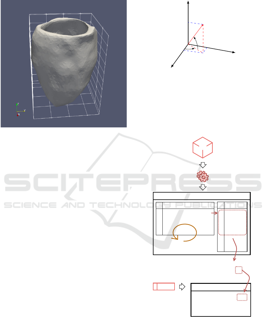
An example of a model build following the meth-

ods described, exported with the original resolution

and default alpha value, is presented in ﬁgure 9.

Left Ventricle Computational Model based on Patients Three-dimensional MRI

159

3434

3232

Y AxisY Axis

3030

3434

2626

3232

Y AxisY Axis

3030

X AxisX Axis

2828

Z AxisZ Axis

X AxisX Axis

3030

Z AxisZ Axis

3030

1010

3232

Figure 9: Renderization of the resulting STL ﬁle.

2.4 Mesh Convertion

In order to use the model in the simulation software, it

is necessary to solve equations that describe the tissue

electrical properties for the whole mesh, therefore the

STL ﬁle must be converted to a tetrahedral mesh, to

deﬁne not only the surface but also the ﬁlling. This

was accomplished using the software TetGen. The

result are a set of ﬁles that list the elements .ele, the

respective nodes .node, facets .face and edges .edges.

The LV model is now made of pyramidal blocks.

2.5 Fibre Orientation

As stated previously there is no information available

about the ﬁbres in the MRI dataset, nevertheless the

way ﬁbres run in the heart muscle has been observed

in in vitro studies and also through Diffusion Tensor

Imaging, therefore is possible to estimate their posi-

tion in a given ventricle, analogously to the method

reported in (Bayer et al., 2012).

Our approach was to follow the geometry de-

scribed in (Khalique and Pennell, 2019), deﬁning the

ﬁbre orientation at each element(tetrahedron) using a

3D vector, that dictates the longitudinal direction the

ﬁbres take from each element.

An example of a vector ~v with the origin at the

centroid of a given element is shown in ﬁgure 10. It is

known that the vector norm is one, therefore by deﬁn-

ing θ and φ and applying trigonometry, it is possible

to determinate the values of v

, v

and v

that deﬁne

the vector.

At the time of the segmentation in MATLAB

Figure 10: Vector ~v representing the ﬁbre orientation at a

given point of the mesh.

when the myocardium is seen in the shape of an an-

nulus, the centre, minimum and maximum radius and

the slice(z value) are register for each slice in a text

ﬁle denominated ’Registration ﬁle’. The sketch of

ﬁgure 11, illustrates how the data necessary for the

following steps is obtained.

Mesh

Nodes

y

z

y

z

y

z

y

z

Repeat for

each element

Elements

node1 node2 node3 node4

TetGen

STL

Centroid

MatLab MatLab

Registration File



cm 

min 

max  

slice

Figure 11: Sketch of the steps required to get the spatial

information, for each element of the mesh.

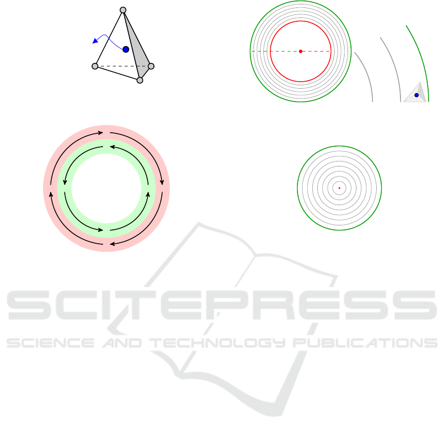
The algorithm written in Python 2.6. starts by

reading the elements from the .ele ﬁle 11, and for each

tetrahedron gets the coordinates of its four nodes from

the .node ﬁle, and calculates the centroid, ﬁgure 12.

During the next steps the volume will have to be

BIOIMAGING 2020 - 7th International Conference on Bioimaging

160

a b

Centroid

Figure 12: Tetrahedron with nodes a,b,c,d and the calcu-

lated centroid.

Figure 13: The ﬁbers closer to the outer border of the mus-

cle run.

imagined as a stack of slices as it was during the seg-

mentation. The closer 2D slice value from the regis-

tration ﬁle to the z coordinate of the centroid will be

attributed to this element. All the calculations will be

made considering the centroid a point in one of the

2D plans, placed at the annulus.

When the left ventricle contracts to pump the

blood it does it by torsion, due to the fact that the

muscle ﬁbres run in opposite directions at the inner -

endocardium - and outer layers - epicardium - as ex-

empliﬁed in ﬁgure 13.

In reality the ﬁbres slope varies according to their

distance to the borders, the ones at the endocardium

do an angle with the horizontal plan that we will con-

sider approximately -60

and it increases along the

muscle till the last layer where we will consider the

angle to measure 60

Deﬁned by an input variable, a number of circum-

ference radius between the minimum (r

min

) and max-

imum (r

max

) radius is saved in an array, imagining the

shape is layered as an onion, the scheme in ﬁgure 14

demonstrates a slice divided in six layers and a cen-

troid positioned at the outermost. At the bottom slices

of the ventricular apex, the minimum radius is consid-

ered zero, ﬁgure 15.

Knowing the angle the vector does with the xy

plan is a value in { -60 : 60 }, going from the out-

ermost circle to the inner, each radius is matched

with an angle θ, according to its position in the ar-

max

min

Figure 14: Left: Myocardium split in six layers deﬁned by

ﬁve radius between r

min

and r

max

Right: tetrahedra with

centroid at the outermost layer.

Figure 15: At the apex r

min

is zero.

ray, which translates in its distance from the centre.

The distance between the centroid and the centre is

matched with the closer radius from the array, and

the θ angle from the orientation vector is therefore as-

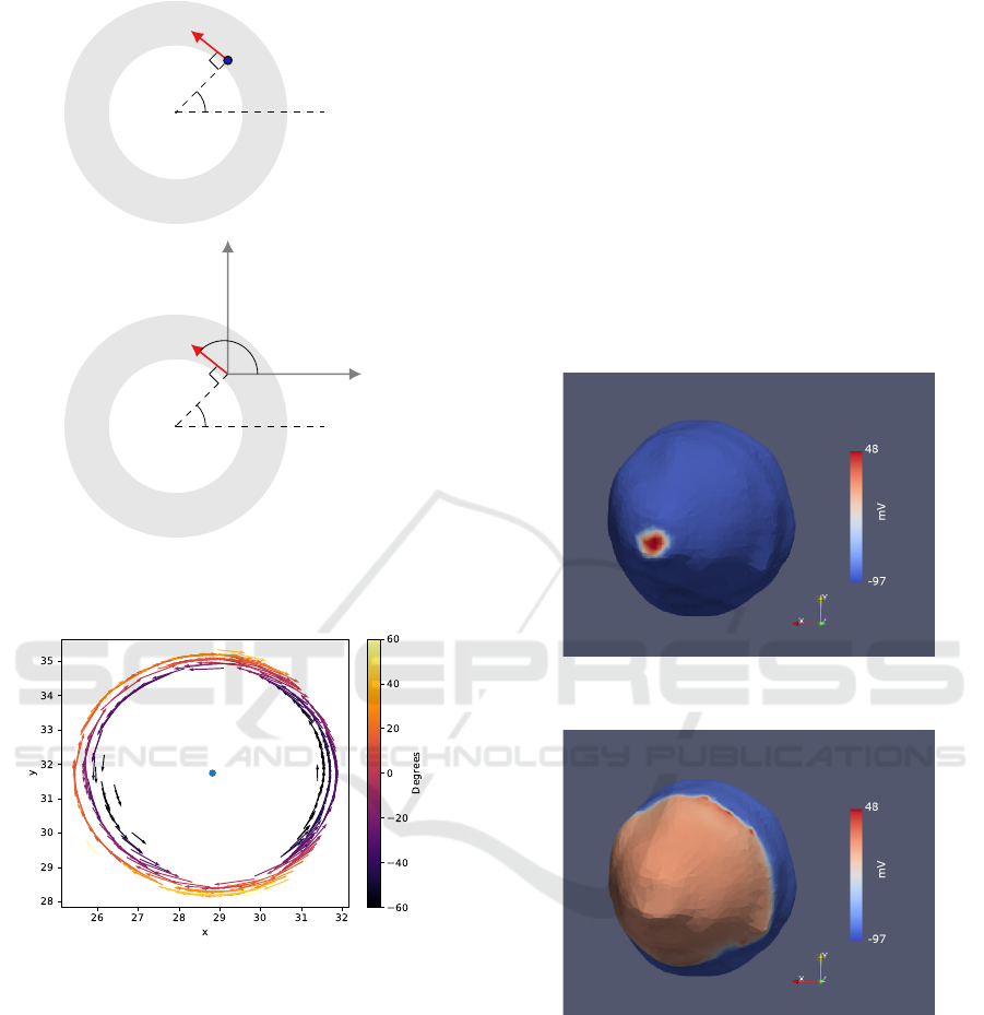
signed. For an element which centroid is located at an

inner layer, the angle φthe vector does with the x axis

is the angle α between the line that connects the cen-

troid with the centre of mass and the vertical line that

crosses the centre of mass, plus 90

. As the scheme

of ﬁgure 16.

For the outer layers, that is when the respective

angle θ is positive, the logic is the same, changing

only the sum of 90

for a subtraction. Considering

the slice of the myocardium a perfect circle, the ﬁbres

as in ﬁgure 13.

Now returning to the 3D system to calculate the

vector third coordinate we know that~v = 1 and both θ

and φ angles, applying the rules of trigonometry to the

scheme in ﬁgure 10 the three coordinates of the vector

can be calculated by the three equations bellow.

x = cos(θ) ∗ cos(φ) (1)

y = cos(θ) ∗ sin(φ) (2)

z = sin(θ) (3)

This logic is followed for every element of the

mesh, the plot of the the resulting orientation vectors

for one of the slices, considering only the 2D plan by

setting z = 0 is presented in ﬁgure 17.

Left Ventricle Computational Model based on Patients Three-dimensional MRI

161

element centroid

y = y

Figure 16: Direction of the vector considering only the xy

plan for an element which centroid is located at an inner

layer.

Figure 17: 2D plot of the orientation vectors for one slice,

where is visible that that the vectors closer to the centre

(blue dot) run anticlockwise and the rest clockwise. From

the colormapping its understood that the inner vectors make

negative angles with the horizontal xy plan, in 3D, and that

this angle gets larger with the proximity to the outer border.

3 RESULTS

To test the model by running electrical simulations, it

was decided to work with the open source software

CHASTE, developed at Oxford University, as it in-

tegrates all the necessary libraries to solve electrical

activation problems on biological tissue, offers ﬂex-

ibility and keeps being improved by the community.

The cardiac module is capable of recreating the exci-

tation signal propagation throughout adjacent neigh-

bouring cells, using a set of parameters that the user

can deﬁne (Mirams et al., 2013).

3.1 Simulation

A simulation ran in monodomain, using the Luo-

Rudy Backward Euler ionic model and intracellular

conductivities of be 3,75 mS/cm for the longitudi-

nal direction and 2.14 mS/cm for transversal and nor-

mal. Considering the tissue homogeneous, applying

a stimuli of -80.000uA at the apex, pictured in ﬁgure

18, after 80 ms the activation spread throughout the

ventricle, as shown in ﬁgure 19.

Figure 18: Spherical stimuli at the apex of the smoothed

model.

Figure 19: Extension of the activation wave after 90 ms.

4 CONCLUSION

Several research groups have been developing paral-

lel functional models of the heart, however most of

the solutions make use of high performance comput-

ers. The approach described in this work intends to

make use of tools available for free or with student

licences. We have proved that it is possible to manip-

ulate the medical images incorporating, in our code,

functions available in MATLAB, plus a couple shared

BIOIMAGING 2020 - 7th International Conference on Bioimaging

162

by the community, resulting in an accurate computa-

tional model of the LV. These are promising results

for the possibility of using non invasive imaging of

human cardiac electrical activity for risk assessments

in diagnostics.

The next logic step is to map different conduc-

tivities accordingly to the intensity levels visible on

contrast-enhanced MRI, allowing to perform virtual

electrophysiologic studies. In order to accomplish

this, the registration process during the segmentation

must be replaced by a more accurate method capa-

ble of mapping the velocities into a model that must

be already a ﬁlled volume, unlike the surface one de-

scribed here.

ACKNOWLEDGEMENTS

This work is part of a project co-funded by Fundac¸

para a Ci

encia e Tecnologia and Compta SA Por-

tugal under the studentship PD/BDE/131399/2017

Ref.CRM:0008003

REFERENCES

Auricchio, Angelo, Singh, Jagmeet, Rademakers, F. E., ed-

itor (2012). Cardiac Imaging in Electrophysiology.

Bayer, J. D., Blake, R. C., Plank, G., and Trayanova,

N. A. (2012). A novel rule-based algorithm for as-

signing myocardial ﬁber orientation to computational

heart models. Annals of biomedical engineering,

40(10):2243–54.

De Maria, E., Aldrovandi, A., Borghi, A., Modonesi, L.,

and Cappelli, S. (2017). Cardiac magnetic resonance

imaging: Which information is useful for the arrhyth-

mologist? World journal of cardiology, 9(10):773–

786.

Di Yu, Dongping Du, Hui Yang, and Yicheng Tu (2014).

Parallel computing simulation of electrical excitation

and conduction in the 3D human heart. In 2014 36th

Annual International Conference of the IEEE Engi-

neering in Medicine and Biology Society, pages 4315–

4319. IEEE.

Holcombe, S. (2011). stlwrite - write ascii or binary stl ﬁles.

Retrieved May 4, 2018.

Khalique, Z. and Pennell, D. (2019). Diffusion tensor car-

diovascular magnetic resonance. Postgraduate medi-

cal journal, 95(1126):433–438.

Kroon, D.-J. (2010). stlwrite - write ascii or binary stl ﬁles.

Retrieved March 26, 2010.

Mirams, G. R., Arthurs, C. J., Bernabeu, M. O., Bordas,

R., Cooper, J., Corrias, A., Davit, Y., Dunn, S.-J.,

Fletcher, A. G., Harvey, D. G., Marsh, M. E., Osborne,

J. M., Pathmanathan, P., Pitt-Francis, J., Southern, J.,

Zemzemi, N., and Gavaghan, D. J. (2013). Chaste: An

Open Source C++ Library for Computational Phys-

iology and Biology. PLoS Computational Biology,

9(3):e1002970.

Tse, G. (2016). Mechanisms of cardiac arrhythmias. Jour-

nal of Arrhythmia, 32(2):75–81.

Left Ventricle Computational Model based on Patients Three-dimensional MRI

163